6. Manual.

6.1. First steps.

6.1.1. Starting the calculations.

All the calculations must start with the Begin command. This command defines the size of the square grid, the grid dimension and the wave length of the field.Before any LightPipes commands the LightPipes package must be imported in your Python script. It is very convenient to use units. Units are included in the LightPipes package.

>>> from LightPipes import *
>>> GridSize = 30*mm
>>> GridDimension = 5
>>> lambda_ = 500*nm #lambda_ is used because lambda is a Python build-in function.
>>> Field = Begin(GridSize, lambda_, GridDimension)
>>> print(Field.field)
[[1.+0.j 1.+0.j 1.+0.j 1.+0.j 1.+0.j]
 [1.+0.j 1.+0.j 1.+0.j 1.+0.j 1.+0.j]
 [1.+0.j 1.+0.j 1.+0.j 1.+0.j 1.+0.j]
 [1.+0.j 1.+0.j 1.+0.j 1.+0.j 1.+0.j]
 [1.+0.j 1.+0.j 1.+0.j 1.+0.j 1.+0.j]]

The use of Begin to define a uniform field with intensity 1 and phase 0.

(Source code, png, hires.png, pdf)

A two dimensional array will be defined containing the complex numbers with the real and imaginary parts equal to one and zero respectively.

6.1.2. The dimensions of structures.

The field structures in LightPipes are two dimensional arrays of complex numbers. For example a grid with 256x256 points asks about 1Mb of memory. 512x512 points ask more then 4Mb and 1024x1024 16Mb. Some commands, however need more memory because internal arrays are necessary. Grids up to 2000 x 2000 points are possible with common PC’s and laptops.

6.1.3. Apertures and screens.

The simplest component to model is an aperture. There are three different types of apertures:

The circular aperture: CircAperture(R, xs, ys, Field)
The rectangular aperture: RectAperture(wx, wy, xs, ys, phi, Field)
The Gaussian diaphragm: GaussAperture(R, xs, ys, T, Field)

Where R=radius, xs and ys are the shift in x and y direction respectively, phi is a rotation and T is the centre transmission of the Gaussian aperture. In addition, there are three commands describing screens: CircScreen (inversion of the circular aperture), RectScreen, (inversion of the rectangular aperture) and GaussScreen (inversion of the gauss aperture).

from LightPipes import *
import matplotlib.pyplot as plt

GridSize = 10*mm
GridDimension = 128
lambda_ = 500*nm #lambda_ is used because lambda is a Python build-in function.

R=2.5*mm #Radius of the aperture
xs=1*mm; ys=1*mm#shift of the aperture

Field = Begin(GridSize, lambda_, GridDimension)
Field=CircAperture(R,xs,ys,Field)
I=Intensity(0,Field)

plt.imshow(I); plt.axis('off')
plt.show()

(Source code, png, hires.png, pdf)

Fig. 1. Example of the application of a circular aperture.

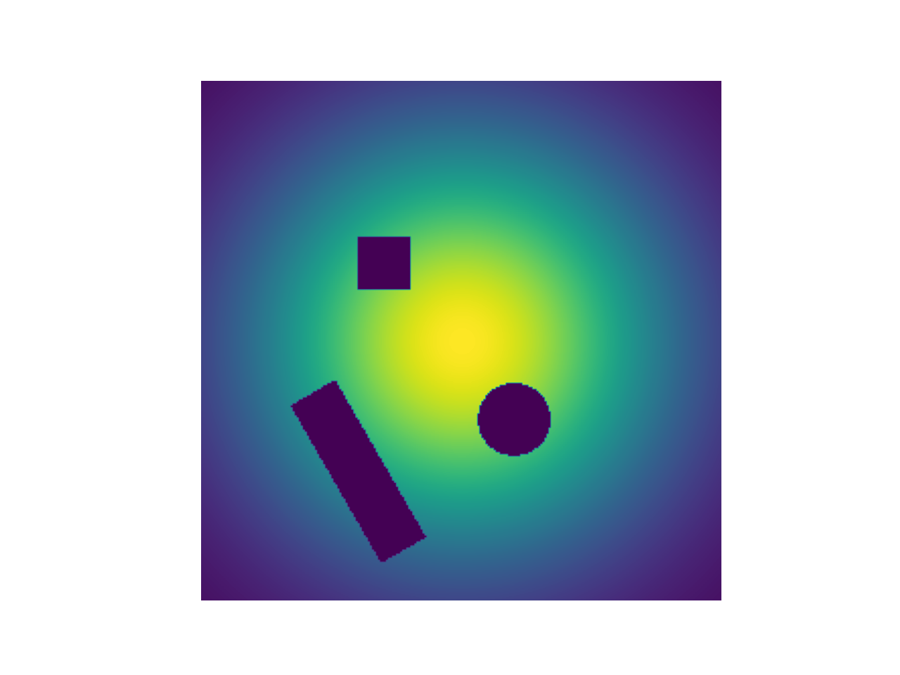
All kinds of combinations of circular, rectangular and Gaussian apertures and screens can be made:

from LightPipes import *
import matplotlib.pyplot as plt

GridSize = 10*mm
GridDimension = 256
lambda_ = 1000*nm #lambda_ is used because lambda is a Python build-in function.

R=2.5*mm #Radius of the aperture
xs=1*mm; ys=1*mm#shift of the aperture

Field = Begin(GridSize, lambda_, GridDimension)
Field=CircScreen(0.7*mm,1*mm,1.5*mm,Field)
Field=RectScreen(1*mm,1*mm,-1.5*mm,-1.5*mm,-0.002,Field)
Field=RectScreen(1*mm,3.5*mm,-2*mm,2.5*mm,30,Field)
Field=GaussAperture(4*mm,0,0,1,Field)
I=Intensity(0,Field)

plt.imshow(I); plt.axis('off')
plt.show()

(Source code, png, hires.png, pdf)

Fig. 2. The use of screens and apertures.

6.1.4. Graphing and visualisation.

In figure 1 and 2 the intensity of the field is calculated after aperturing ‘Field’ with the Intensity command using option 0, which means that no normalization is applied. Alternatives are option 1: normalization to 1 and option 2: normalization to 255 for displaying gray-values (not often needed). Use has been made of the package “matplotlib” which can be installed by typing at the python prompt:

>>> pip install matplotlib

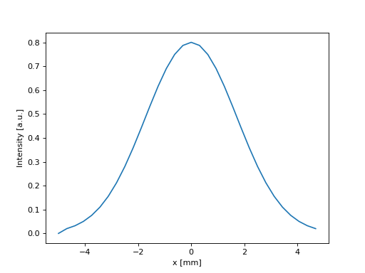
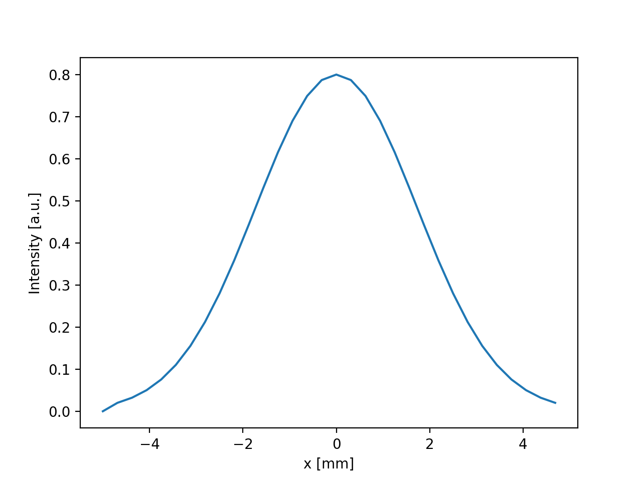
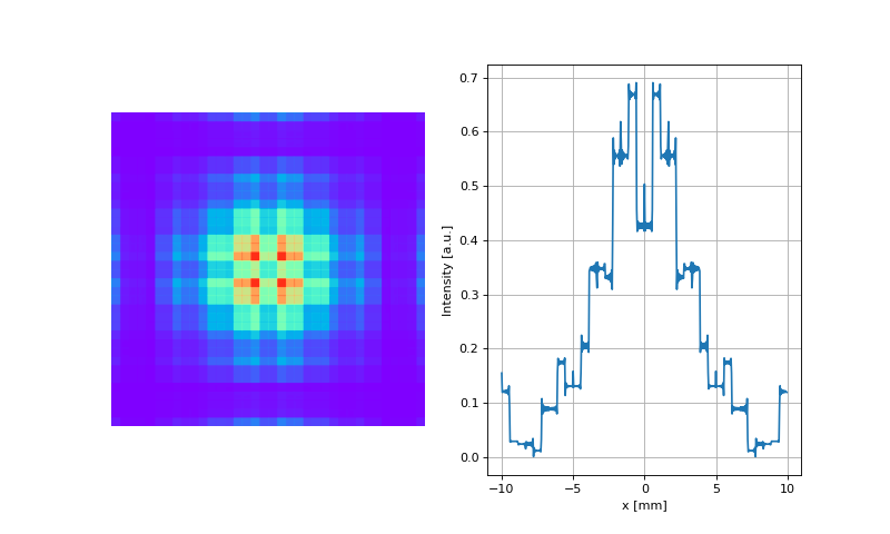
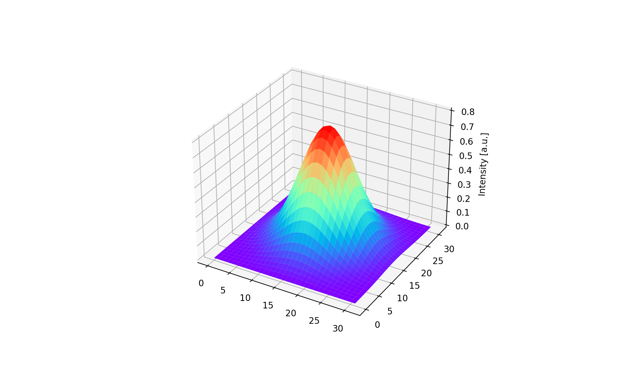
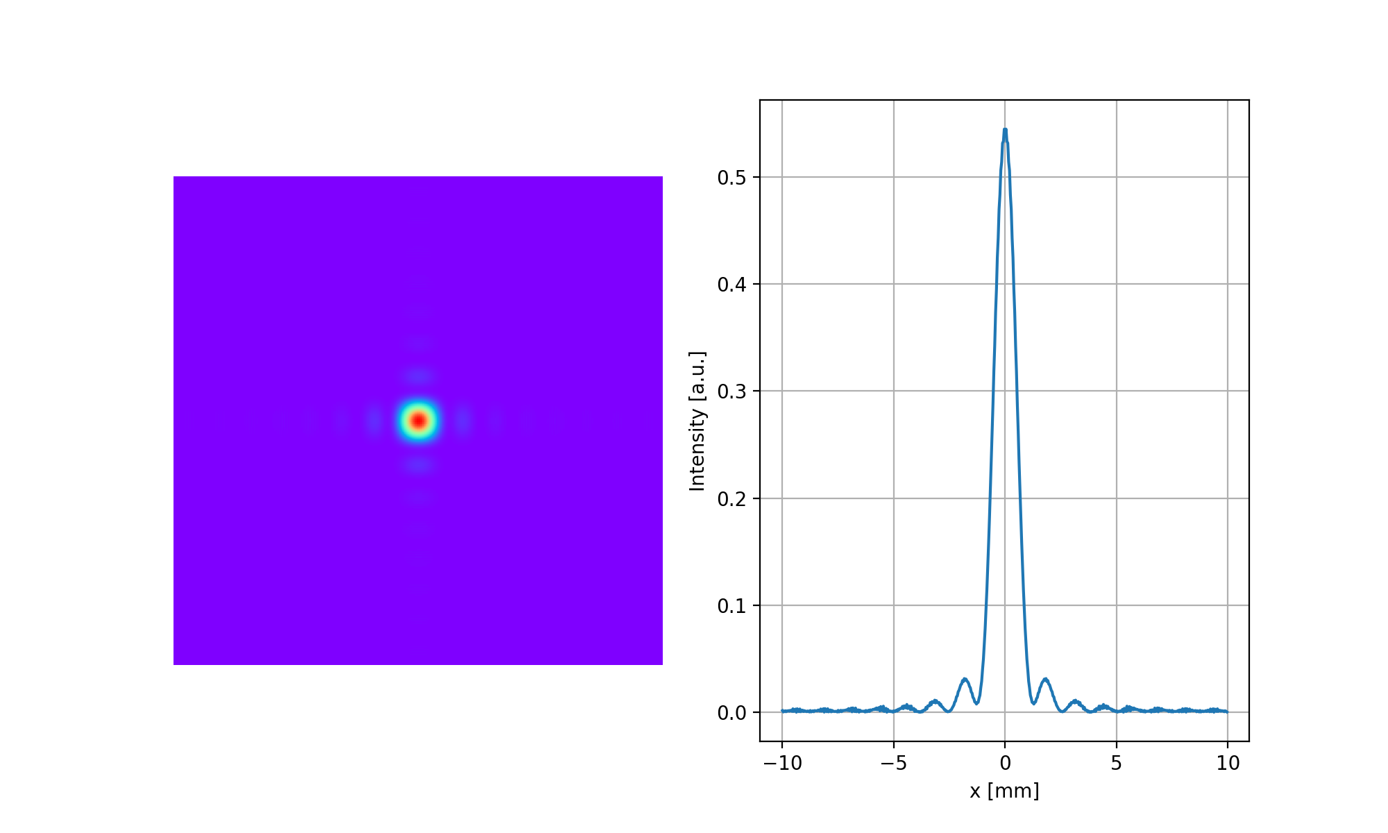
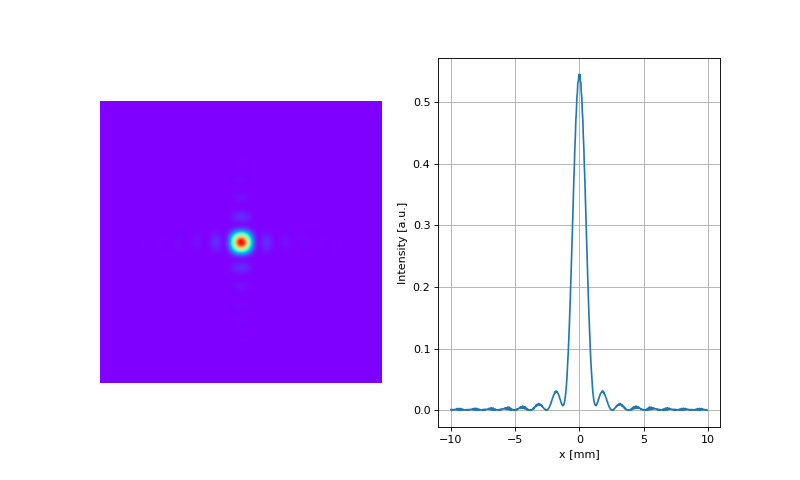
With the command Interpol you can reduce the grid dimension of the field speeding up subsequent plotting considerably, especially when dealing with 3d surface plots. This is illustrated in figure 3. In figure 3 we also plotted the cross section of the beam in a two dimensional XY plot. For this we have to define an integer, i, ranging from 1 to the grid dimension. This integer must be used to define the element of the (square) array, I, which is used for the vertical axis of the XY plot. Use has been made of the “numpy” package which can be installed by typing at the python prompt:

>>> pip install numpy

from LightPipes import *
import matplotlib.pyplot as plt
from mpl_toolkits.mplot3d import Axes3D
import numpy as np

GridSize = 10*mm
GridDimension = 128
lambda_ = 1000*nm #lambda_ is used because lambda is a Python build-in function.

R=2.5*mm
xs=0*mm; ys=0*mm
T=0.8

Field = Begin(GridSize, lambda_, GridDimension)
Field=GaussAperture(R,xs,ys,T,Field)
NewGridDimension=int(GridDimension/4)
Field=Interpol(GridSize,NewGridDimension,0,0,0,1,Field)
I=Intensity(0,Field)
I=np.array(I)

#plot cross section:
x=[]
for i in range(NewGridDimension):
    x.append((-GridSize/2+i*GridSize/NewGridDimension)/mm)
plt.plot(x,I[int(NewGridDimension/2)])
plt.xlabel('x [mm]');plt.ylabel('Intensity [a.u.]')
plt.show()

(Source code, png, hires.png, pdf)

#3d plot:
X=range(NewGridDimension)
Y=range(NewGridDimension)
X, Y=np.meshgrid(X,Y) 
fig=plt.figure(figsize=(10,6))
ax = plt.axes(projection='3d')
ax.plot_surface(X, Y,I,
                rstride=1,
                cstride=1,
                cmap='rainbow',
                linewidth=0.0,
                )
ax.set_zlabel('Intensity [a.u.]')
plt.show()

(png, hires.png, pdf)

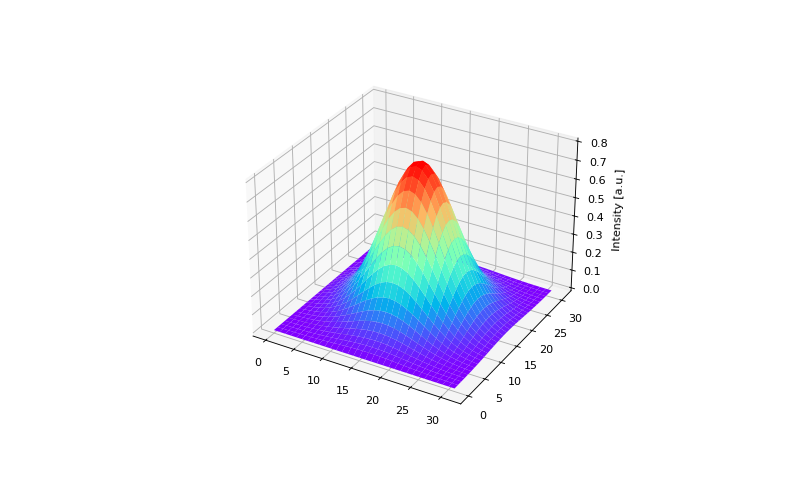
Fig. 3. The use of XY-plots and surface plots to present your simulation results. Note the usage of Interpol to reduce the grid dimension for a faster surface plot.

For more see: https://matplotlib.org

6.2. Free space propagation.

There are four different possibilities for modelling the light propagation in LightPipes.

6.2.1. FFT propagation (spectral method).

Let us consider the wave function \(U\) in two planes: \(U(x,y,0\)) and \(U(x,y,z)\). Suppose then that \(U(x,y,z)\) is the result of propagation of \(U(x,y,0)\) to the distance \(z\) , with the Fourier transforms of these two (initial and propagated ) wave functions given by \(A(\alpha,\beta,0)\) and \(A(\alpha,\beta,z)\) correspondingly. In the Fresnel approximation, the Fourier transform of the diffracted wave function is related to the Fourier transform of the initial function via the frequency transfer characteristic of the free space \(H( \alpha,\beta,z)\) , given by 1 2 :

(1)\[H=\frac{A(\alpha, \beta, z)}{A(\alpha, \beta, 0)}=\exp \big\{ {{-ikz(1-\alpha^2-\beta^2)}^{1/2}}\big\}\]

where:

(2)\[A(\alpha, \beta,0)= \int \int_{ -\infty} ^{ \infty} U(x,y,0)exp{\{-ikz(\alpha x+\beta y)}\}dxdy\]

(3)\[A(\alpha, \beta,z)= \int \int_{ -\infty} ^{ \infty} U(x,y,z)exp{\{-ikz(\alpha x+\beta y)}\}dxdy\]

Expressions (1), (2), and (3) provide a symmetrical relation between the initial and diffracted wave functions in the Fresnel approximation. Applied in the order (2) \(\rightarrow\) (1) \(\rightarrow\) (3) they result in the diffracted wave function, while being applied in the reversed order they allow for reconstruction of the initial wave function from the result of diffraction. We shall denote the forward and the reversed propagation operations defined by expressions (1), (2) and (3) with operators \(L^+\) and \(L^-\) respectively. The described algorithm can be implemented numerically using Fast Fourier Transform (FFT) 2 3 on a finite rectangular grid with periodic border conditions. It results in a model of beam propagation inside a rectangular wave guide with reflective walls. To approximate a free-space propagation, wide empty guard bands have to be formed around the wave function defined on a grid. To eliminate the influence of the finite rectangular data window, Gaussian amplitude windowing in the frequency domain should be applied, see 2 3 for extensive analysis of these computational aspects. The simplest and fastest LightPipes command for propagation is Forvard. (The ‘v’ is a type error made on purpose!) It implements the spectral method described by 1 2 3 . 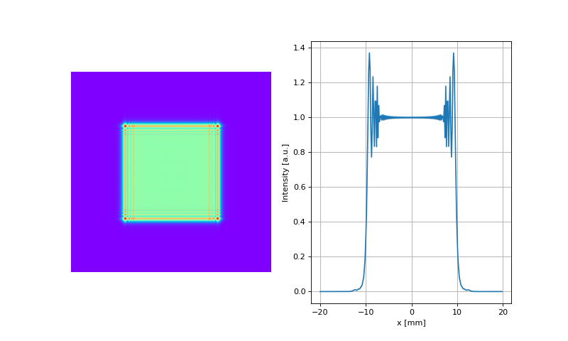The syntax is simple, for example if you want to filter your field through a 1cm aperture and then propagate the beam 1m forward, you type the following commands:

from LightPipes import *
import matplotlib.pyplot as plt

Field=Begin(20*mm, 1*um, 256)
Field = CircAperture(5*mm, 0, 0, Field)
Field = Forvard(1*m, Field)
I = Intensity(0,Field)

x=[]
for i in range(256):
    x.append((-20*mm/2+i*20*mm/256)/mm)

fig=plt.figure(figsize=(15,6))
ax1 = fig.add_subplot(121)
ax2 = fig.add_subplot(122)
ax1.imshow(I,cmap='rainbow'); ax1.axis('off')
ax2.plot(x,I[128]);ax2.set_xlabel('x [mm]');ax2.set_ylabel('Intensity [a.u.]')
ax2.grid('on')
plt.show()

(Source code, png, hires.png, pdf)

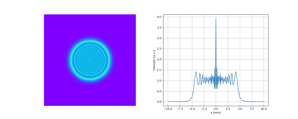
Fig. 4. The result of the propagation: density and cross section intensity plots.

We see the diffraction effects, the intensity distribution is not uniform anymore. The algorithm is very fast in comparison with direct calculation of diffraction integrals. Features to be taken into account: The algorithm realises a model of light beam propagation inside a square wave guide with reflecting walls positioned at the grid edges. To approximate a free space propagation, the intensity near the walls must be negligible small. Thus the grid edges must be far enough from the propagating beam. Neglecting these conditions will cause interference of the propagating beam with waves reflected from the wave guide walls. As a consequence of the previous feature, we must be extremely careful propagating the plane wave to a distance comparable with \(D^2/\lambda\) where \(D\) is the diameter (or a characteristic size) of the beam, and \(\lambda\) is the wavelength. To propagate the beam to the far field (or just far enough) we have to choose the size of our grid much larger than the beam itself, in other words we define the field in a grid filled mainly with zeros. The grid must be even larger when the beam is aberrated because the divergent beams reach the region border sooner.

Due to these two reasons the commands:

from LightPipes import *
import matplotlib.pyplot as plt

Field=Begin(20*mm, 1*um, 256)
Field = RectAperture(20*mm,20*mm,0, 0,0, Field)
Field = Forvard(1*m, Field)
I = Intensity(0,Field)

x=[]
for i in range(256):
    x.append((-20*mm/2+i*20*mm/256)/mm)

fig=plt.figure(figsize=(15,6))
ax1 = fig.add_subplot(121)
ax2 = fig.add_subplot(122)
ax1.imshow(I,cmap='rainbow'); ax1.axis('off')
ax2.plot(x,I[128]);ax2.set_xlabel('x [mm]');ax2.set_ylabel('Intensity [a.u.]')
ax2.grid('on')
plt.show()

(Source code, png, hires.png, pdf)

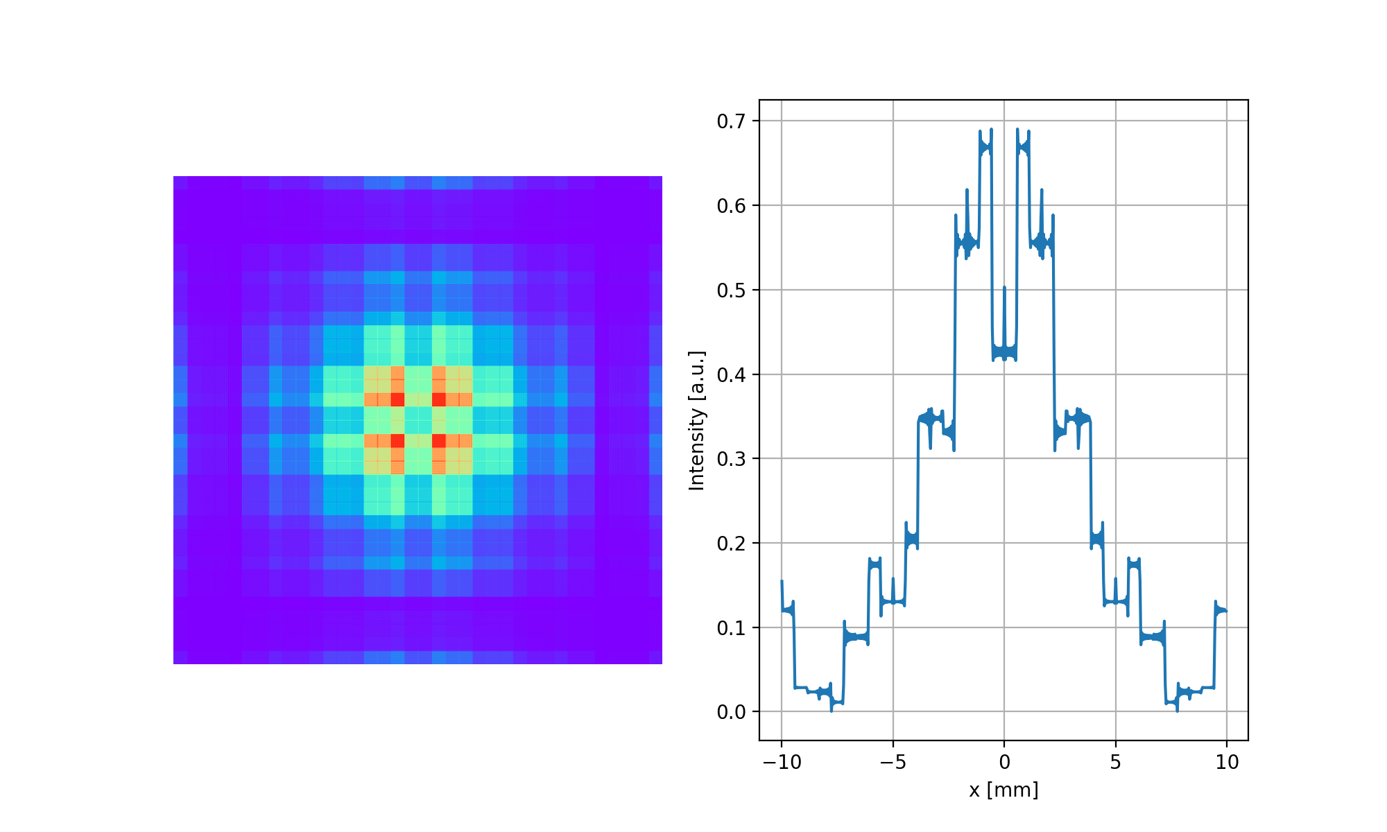
make no sense. The cross section of the beam (argument of RectAperture) equals to the section of the grid (the first argument of Begin), so we have a model of light propagation in a wave guide but not in a free space. One has to put:

from LightPipes import *
import matplotlib.pyplot as plt

Field=Begin(40*mm, 1*um, 256)
Field = RectAperture(20*mm,20*mm,0, 0,0, Field)
Field = Forvard(1*m, Field)
I = Intensity(0,Field)

x=[]
for i in range(256):
    x.append((-40*mm/2+i*40*mm/256)/mm)

fig=plt.figure(figsize=(10,6))
ax1 = fig.add_subplot(121)
ax2 = fig.add_subplot(122)
ax1.imshow(I,cmap='rainbow'); ax1.axis('off')
ax2.plot(x,I[128]);ax2.set_xlabel('x [mm]');ax2.set_ylabel('Intensity [a.u.]')
ax2.grid('on')
plt.show()

(Source code, png, hires.png, pdf)

for propagation in the near field, and may be:

from LightPipes import *
import matplotlib.pyplot as plt

Field=Begin(400*mm, 1*um, 512)
Field = RectAperture(20*mm,20*mm,0, 0,0, Field)
Field = Forvard(500*m, Field)
I = Intensity(0,Field)

x=[]
for i in range(512):
    x.append((-20*mm/2+i*20*mm/512)/mm)

fig=plt.figure(figsize=(10,6))
ax1 = fig.add_subplot(121)
ax2 = fig.add_subplot(122)
ax1.imshow(I,cmap='rainbow'); ax1.axis('off')
ax2.plot(x,I[256]);ax2.set_xlabel('x [mm]');ax2.set_ylabel('Intensity [a.u.]')
ax2.grid('on')
plt.show()

(Source code, png, hires.png, pdf)

for far field propagation. If we compare the result of the previous example with the result of:

from LightPipes import *
import matplotlib.pyplot as plt

Field=Begin(60*mm, 1*um, 512)
Field = RectAperture(20*mm,20*mm,0, 0,0, Field)
Field = Forvard(500*m, Field)
I = Intensity(0,Field)

x=[]
for i in range(512):
    x.append((-20*mm/2+i*20*mm/512)/mm)

fig=plt.figure(figsize=(10,6))
ax1 = fig.add_subplot(121)
ax2 = fig.add_subplot(122)
ax1.imshow(I,cmap='rainbow'); ax1.axis('off')
ax2.plot(x,I[256]);ax2.set_xlabel('x [mm]');ax2.set_ylabel('Intensity [a.u.]')
ax2.grid('on')
plt.show()

(Source code, png, hires.png, pdf)

we’ll see the difference.

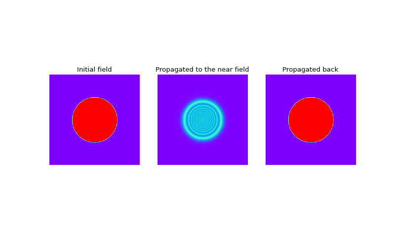
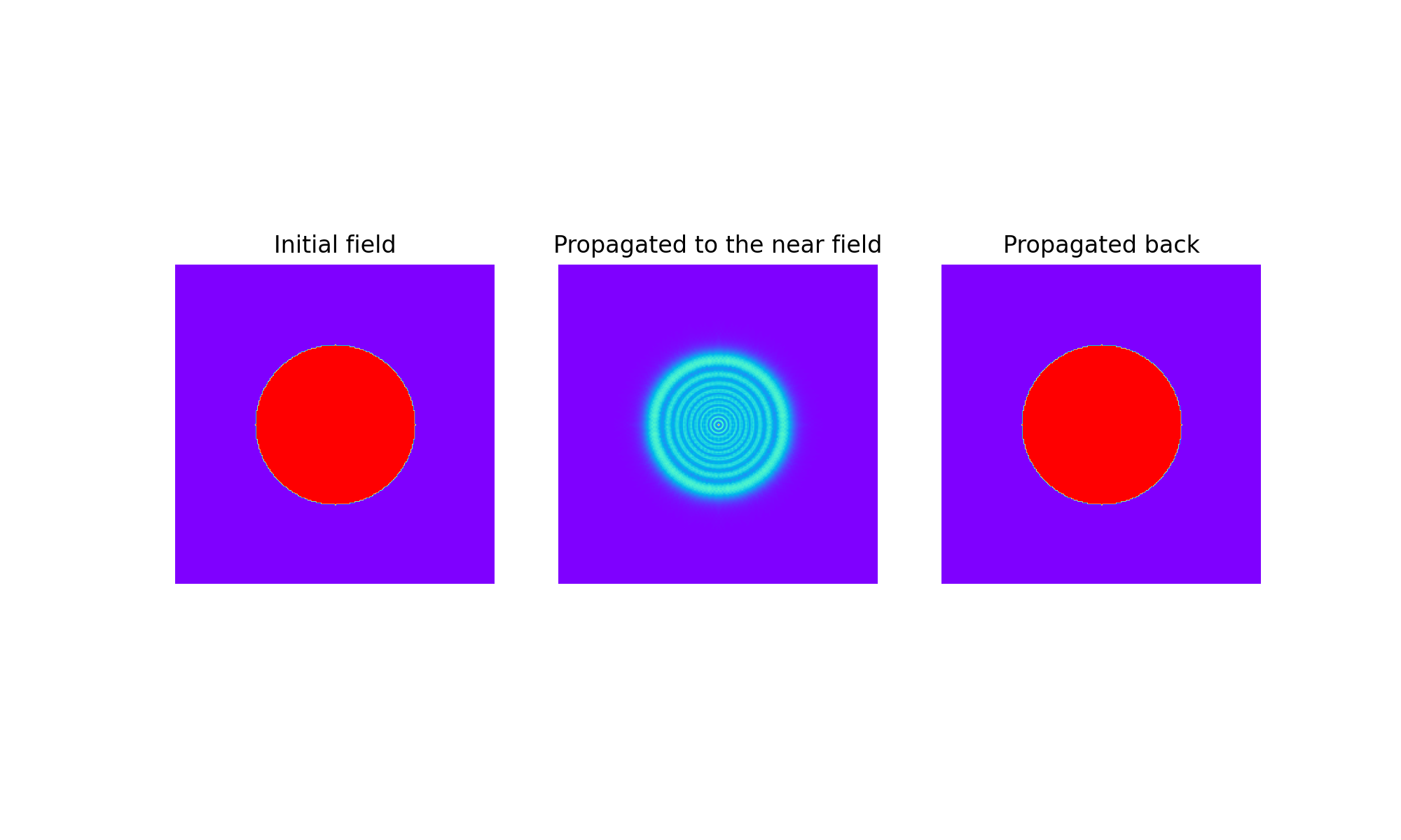
We have discussed briefly the drawbacks of the FFT algorithm. The good thing is that it is very fast, works pretty well if properly used, is simple in implementation and does not require the allocation of extra memory. In LightPipes a negative argument may be supplied to Forvard. It means that the program will perform “propagation back” or in other words it will reconstruct the initial field from the one diffracted. For example:

from LightPipes import *
import matplotlib.pyplot as plt

Field=Begin(100*mm, 1*um, 256)
Field = CircAperture(25*mm,0, 0, Field)
I0=Intensity(0,Field)
Field = Forvard(30*m, Field)
I1 = Intensity(0,Field)
Field = Forvard(-30*m, Field)
I2 = Intensity(0,Field)

x=[]
for i in range(512):
    x.append((-20*mm/2+i*20*mm/512)/mm)

fig=plt.figure(figsize=(10,6))
ax1 = fig.add_subplot(131)
ax2 = fig.add_subplot(132)
ax3 = fig.add_subplot(133)
ax1.imshow(I0,cmap='rainbow'); ax1.axis('off'); ax1.set_title('Initial field')
ax2.imshow(I1,cmap='rainbow'); ax2.axis('off'); ax2.set_title('Propagated to the near field')
ax3.imshow(I2,cmap='rainbow'); ax3.axis('off'); ax3.set_title('Propagated back')
plt.show()

(Source code, png, hires.png, pdf)

Fig. 5. The initial filed, the field propagated to the near field and the field propagated back

6.2.2. Direct integration as a convolution: FFT approach.

Another possibility of a fast computer implementation of the operator \(L^+\) is free from many of the drawbacks of the described spectral algorithm. The operator \(L^+\) may be numerically implemented with direct summation of the Fresnel-Kirchoff diffraction integral:

(4)\[U(x_1,y_1,z)=\frac{k}{2\pi iz} \int \int U(x,y,0)\exp \big\{ik\frac{(x-x_1)^2+(y-y_1)^2}{2 z}\big\}dxdy\]

with functions \(U(x,y,0)\) and \(U(x,y,z)\) defined on rectangular grids. This integral may be converted into a convolution form which can be efficiently computed using FFT 4 , [f#5]_ . This method is free from many drawbacks of the spectral method given by the sequence (3) \(\rightarrow\) (2) \(\rightarrow\) (4) although it is still very fast due to its use of FFT for computing of the integral sums.

We’ll explain this using a two-dimensional example, following 4, p.100. Let the integral be defined in a finite interval \(–L/2\cdots L/2\):

(5)\[U(x_1,z)= \sqrt{ \frac{k}{2\pi iz}} \int _{-L/2}^{L/2} U(x,0)\exp \big\{ik\frac{(x-x_1)^2}{2 z}\big\}dx\]

Replacing the functions U(x) and U(x1) with step functions Uj and Um, defined in the sampling points of the grid with j=0…N, and m=0…N we convert the integral (5.5) to the form:

(6)\[U_m= \sqrt{ \frac{k}{2\pi iz}} \sum_{j=1}^{N-1}U_j \int _{x_j-0.5}^{x_j+0.5} \exp \big\{ik\frac{(x_m-x)^2}{2 z}\big\}dx + U_0 \int _{x_0}^{0.5} \exp \big\{ik\frac{(x_m-x)^2}{2 z}\big\}dx + U_N \int _{x_N-0.5}^{x_N} \exp \big\{ik\frac{(x_m-x)^2}{2 z}\big\}dx\]

Taking the integrals in (6) we obtain:

(7)\[U_m= \sum_{j=1}^{N-1} U_j K_{mj}+U_0K_{m0}+U_NK_{mN}\]

where: \(K_{m0}\), \(K_{mj}\) and \(K_{mN}\) are analytical expressed with the help of Fresnel integrals, depending only onto the difference of indices. The summations \(\sum_{j=1}^{N-1} U_j K_{mj}\) can easily be calculated for all indices m as one convolution with the help of FFT.

The command Fresnel implements this algorithm using the trapezoidal rule. It is almost as fast as Forvard (from 2 to 5 times slower), it uses 8 times more memory than Forvard and it allows for “more honest” calculation of near and far-field diffraction. As it does not require any protection bands at the edges of the region, the model may be built in a smaller grid, therefore the resources consumed and time of execution are comparable or even better than that of Forvard. Fresnel does not accept a negative propagation distance. When possible Fresnel has to be used as the main computational engine within LightPipes.

Warning: Fresnel does not produce valid results if the distance of propagation is comparable with (or less than) the characteristic size of the aperture at which the field is diffracted. In this case Forvard or Steps should be used.

6.2.3. Direct integration.

Direct calculation of the Fresnel-Kirchoff integrals is very inefficient in two-dimensional grids. The number of operations is proportional to \(N^4\) , where \(N\) is the grid sampling. With direct integration we do not have any reflection at the grid boundary, so the size of the grid can just match the cross section of field distribution. LightPipes include a program Forward realizing direct integration. Forward has the following features:

arbitrary sampling and size of square grid at the input plane.

arbitrary sampling and size of square grid at the output plane, it means we can propagate the field from a grid containing for example 52 x 52 points corresponding to 4.9 x4 .9 cm to a grid containing 42 x 42 points and corresponding let’s say 8.75 x 8.75 cm.

6.2.4. Finite difference method.

It can be shown that the propagation of the field \(U\) in a medium with complex refractive coefficient \(A\), is described by the differential equation:

(8)\[\frac{\partial^2U}{\partial x^2} + \frac{\partial^2U}{\partial y^2}+2ik \frac{\partial U}{\partial z} +A(x,y,z)U=0\]

To solve this equation, we re-write it as a system of finite difference equations:

(9)\[\frac{U^{k+1}_{i+1,j}-2U^{k+1}_{i,j}+U^{k+1}_{i-1,j}}{\Delta x^2}+\frac{U^{k}_{i,j+1}-2U^{k}_{i,j}+U^{k}_{i,j-1}}{\Delta y^2}+2ik\frac{U^{k+1}_{i,j}-2U^k_{i,j}}{\Delta z}+A^{k+1}_{i,j}U^{k+1}_{i,j}=0\]

Collecting terms we obtain the standard three-diagonal system of linear equations, the solution of which describes the complex amplitude of the light field in the layer \(z+\Delta z\) as a function of the field defined in the layer z:

(10)\[-a_iU^{k+1}_{i-1,j}+c_iU^{k+1}_{i,j}-b_iU^{k+1}_{i+1,j}=f_i\]

where: (we put \(\Delta x=\Delta y=\Delta\) )

(11)\[a_i=b_i=-\frac{1}{\Delta^2}\]

(12)\[c_i=A^{k+1}_{i,j}-\frac{2}{\Delta^2}+\frac{2ik}{\Delta z}\]

(13)\[f_i=\frac{2ik}{\Delta z}U^k_{i,j}-\frac{U^k_{i,j+1}-2U^k_{i,j}+U^k_{i,j-1}}{\Delta^2}\]

The three-diagonal system of linear equations (10) is solved by the standard elimination (double sweep) method, described for example in 1 . This scheme is absolutely stable (this variant is explicit with respect to the index \(i\) and implicit with respect to the index \(j\)). One step of propagation is divided into two sub-steps: the first sub-step applies the described procedure to all rows of the matrix, the second sub-step changes the direction of elimination and the procedure is applied to all columns of the matrix.

The main advantage of this approach is the possibility to take into account uniformly diffraction, absorption (amplification) and refraction. For example, the model of a waveguide with complex three-dimensional distribution of refraction index and absorption coefficient (both are defined as real and imaginary components of the (three-dimensional in general) matrix \(A^k_{i,j}\)) can be built easily.

It works also much faster than all described previously algorithms on one step of propagation, though to obtain a good result at a considerable distance, many steps should be done. As the scheme is absolutely stable (at least for free-space propagation), there is no stability limitation on the step size in the direction \(z.\) Large steps cause high-frequency errors, therefore the number of steps should be determined by trial (increase the number of steps in a probe model till the result stabilizes), especially for strong variations of refraction and absorption inside the propagation path.

Zero amplitude boundary conditions are commonly used for the described system. This, again, creates the problem of the wave reflection at the grid boundary. The influence of these reflections in many cases can be reduced by introducing an additional absorbing layer in the proximity of the boundary, with the absorption smoothly (to reduce the reflection at the absorption gradient) increasing towards the boundary.

In LightPipes for Python 2.1.4 the refraction term is not included into the propagation formulas, instead the phase of the field is modified at each step according to the distribution of the refractive coefficient. This “zero-order” approximation happened to be much more stable numerically than the direct inclusion of refraction terms into propagation formulas. It does not take into account the change of the wavelength in the medium, it does not model backscattering and reflections back on interfaces between different media. Perhaps there are other details to be mentioned. The described algorithm is implemented in the Steps command.

#Focus of a lens.
from LightPipes import*
import numpy as np
from mpl_toolkits.mplot3d import Axes3D
import matplotlib.pyplot as plt

wavelength=632.8*nm;
size=4*mm;
N=100;
N2=50;
R=1.5*mm;
dz=10*mm;
f=50*cm;
n=(1.0 + 0.1j)*np.ones((N,N))

Icross=np.zeros((100,N))
X=range(N)
Z=range(100)
X, Z=np.meshgrid(X,Z)
F=Begin(size,wavelength,N);
F=CircAperture(R,0,0,F);
F=Lens(f,0,0,F);
for i in range(0,100):
  F=Steps(dz,1,n,F);
  I=Intensity(0,F);
  Icross[i][:N]=I[N2][:N]

ax = plt.axes(projection='3d')
ax.plot_surface(X, Z,
        Icross,
        rstride=1,
        cstride=1,
        cmap='rainbow',
        linewidth=0.0,
        )
plt.axis('off')
plt.show()

(Source code, png, hires.png, pdf)

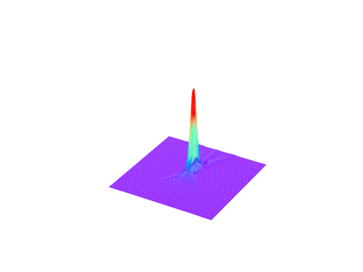
Fig. 6. The use of Steps to calculate the intensity distribution in the focus of a lens.

The Steps command has a built-in absorption layer along the grid boundaries (to prevent reflections), occupying 10% of grid from each side. Steps is the only command in LightPipes allowing for modeling of (three-dimensional) waveguide devices.

Like Forvard, Steps can inversely propagate the field, for example the sequence

Field = Steps( 0.1, 1, n, Field)
Field = Steps(-0.1, 1, n ,Field)

doesn’t change anything in the field distribution. The author has tested this reversibility also for propagation in absorptive/refractive media, examples will follow.

Steps implements scalar approximation, it is not applicable for modeling of waveguide devices in the vector approximation, where two components of the field should be taken into account.

6.3. Splitting and mixing beams.

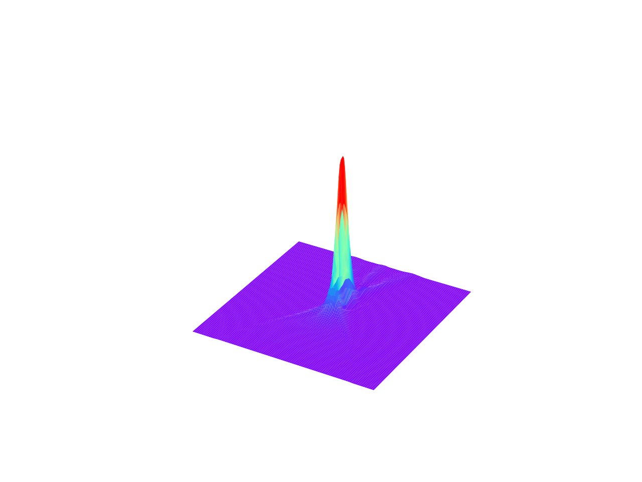
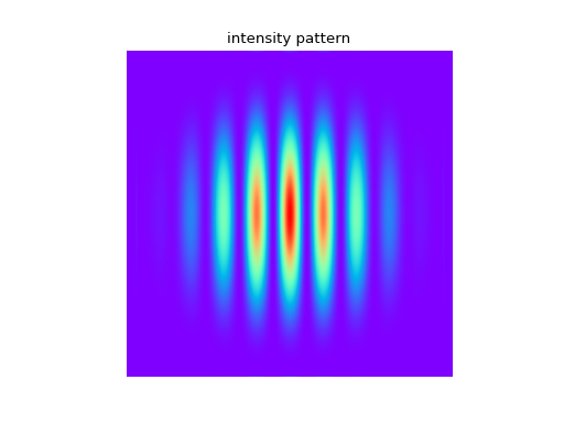
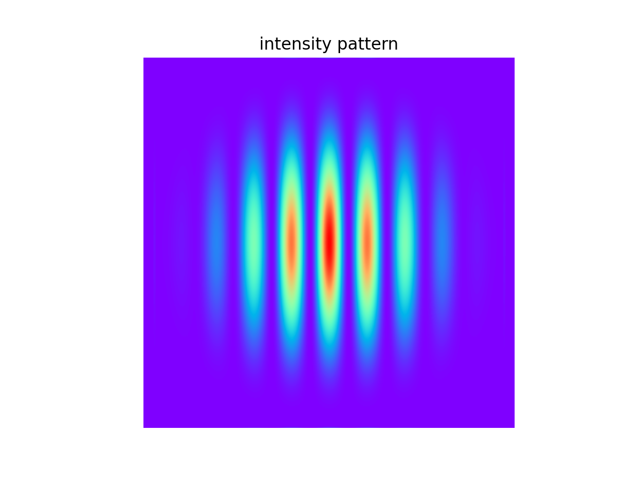
There are two commands in LightPipes which are useful for modelling of interferometers. With IntAttenuator we can split the field structure (amplitude division) - The two obtained fields could be processed separately and then mixed again with the routine BeamMix. In this script we have formed two beams each containing one “shifted” hole. After mixing these two beams we have a screen with two holes: a Young’s interferometer.

from LightPipes import *
import matplotlib.pyplot as plt
import matplotlib.image as mpimg
LPversion
"""
    Young's experiment.
    Two holes with radii, R, separated by, d, in a screen are illuminated by a plane wave. The interference pattern
    at a distance, z, behind the screen is calculated.
"""
print(LPversion)
wavelength=5*um
size=20.0*mm
N=500
z=50*cm
R=0.3*mm
d=1.2*mm

#img=mpimg.imread('Young.png')
#plt.imshow(img); plt.axis('off')

#plt.show()

F=Begin(size,wavelength,N)
F1=CircAperture(R/2.0,-d/2.0, 0, F)
F2=CircAperture(R/2.0, d/2.0, 0, F)    
F=BeamMix(F1,F2)
F=Fresnel(z,F)
I=Intensity(2,F)
plt.imshow(I, cmap='rainbow'); plt.axis('off');plt.title('intensity pattern')
plt.show()

(Source code, png, hires.png, pdf)

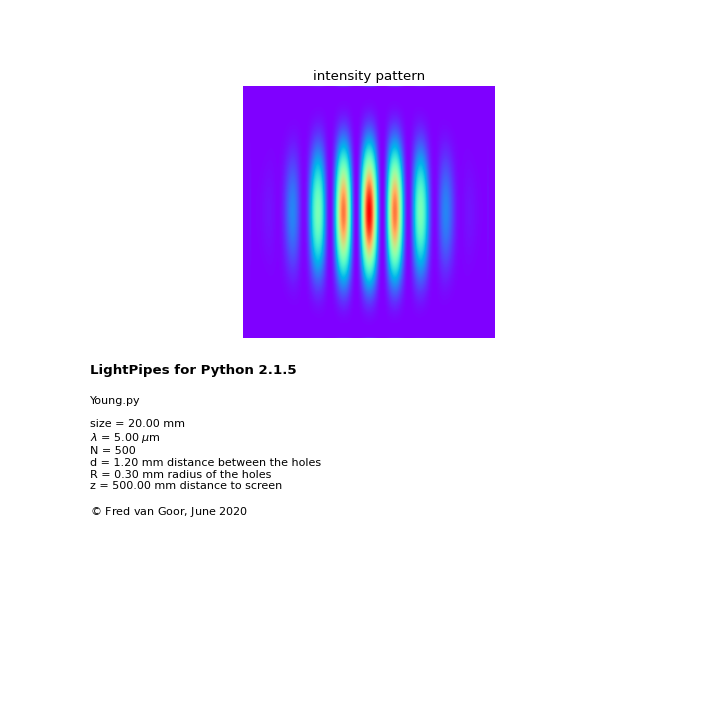
Fig. 7. Young’s interferometer.

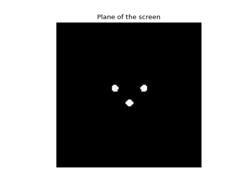
Having the model of the interferometer we can “play” with it, moving the pinholes and changing their sizes. The following models the result of the interference of a plane wave diffracted at three round apertures:

from LightPipes import *
import matplotlib.pyplot as plt

wavelength=550*nm
size=5*mm
N=128
R=0.12*mm
x=0.5*mm
y=0.25*mm
z=75*cm

F=Begin(size,wavelength,N)
F1=CircAperture(R,-x, -y, F)
F2=CircAperture(R, x, -y, F)
F3=CircAperture(R, 0, y, F)  
F=BeamMix(BeamMix(F1,F2),F3)
I0=Intensity(2,F)
F=Fresnel(z,F)
I1=Intensity(2,F)

plt.imshow(I0, cmap='gray'); plt.axis('off');plt.title('Plane of the screen')
plt.show()

(Source code, png, hires.png, pdf)

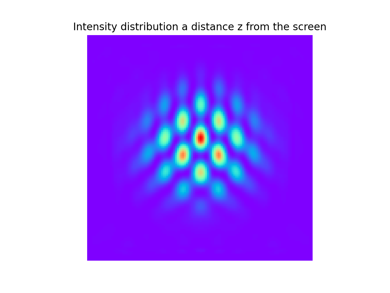
plt.imshow(I1, cmap='rainbow'); plt.axis('off');plt.title('Intensity distribution a distance z from the screen')
plt.show()

(png, hires.png, pdf)

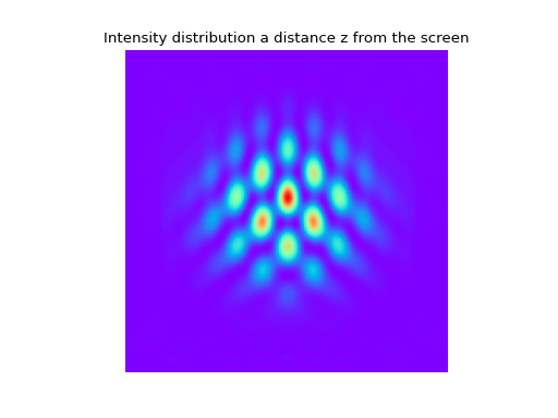
Fig. 8. Intensity distributions in the plane of the screen and 75cm behind the screen.

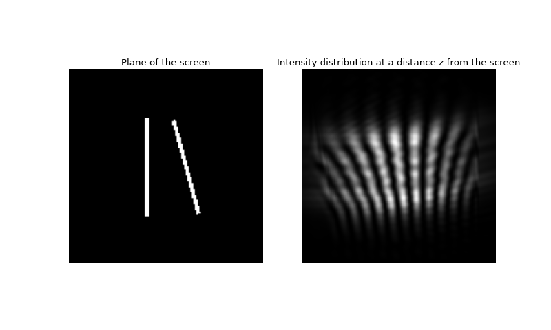
The next interferometer is more interesting:

#! python3

import matplotlib.pyplot as plt
from LightPipes import *

wavelength=550*nm
size=5*mm
N=128
w=0.1*mm
h=2.5*mm
phi=15*rad
x=0.5*mm
z=75*cm

F = Begin(size,wavelength,N)
F1 = RectAperture(w, h,-x,0, 0, F)
F2 = RectAperture(w, h,x,0, phi, F) 
F=BeamMix(F1,F2)
I0=Intensity(2,F)
F=Fresnel(z,F)
I1=Intensity(1,F)

fig=plt.figure(figsize=(10,6))
ax1 = fig.add_subplot(121)
ax2 = fig.add_subplot(122)

ax1.imshow(I0,cmap='gray',aspect='equal');ax1.axis('off'); ax1.set_title('Plane of the screen')
ax2.imshow(I1,cmap='gray',aspect='equal');ax2.axis('off'); ax2.set_title('Intensity distribution at a distance z from the screen')

plt.show()

(Source code, png, hires.png, pdf)

Fig. 9. Intensity distributions in the plane of the screen and 75cm behind the screen.

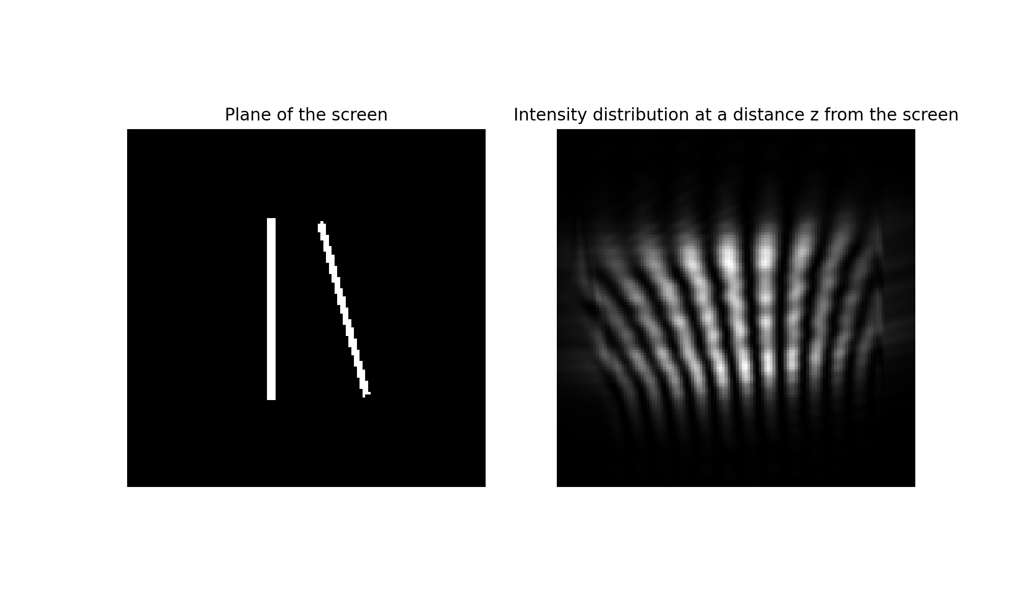
In the last example the intensity distribution is modulated by the wave, reflected from the grid edge, nevertheless it gives a good impression about the general character of the interference pattern. To obtain a better result, the calculations should be conducted in a larger grid or other numerical method should be used. The following example uses a direct integration algorithm (the input and output are in different scales and have different samplings):

#! python3

import matplotlib.pyplot as plt
from LightPipes import *

wavelength=550*nm
size=2.6*mm
N=64
w=0.1*mm
h=2.5*mm
phi=15*rad
x=0.5*mm
z=75*cm
sizenew=5*mm

F = Begin(size,wavelength,N)
F1 = RectAperture(w, h,-x,0, 0, F)
F2 = RectAperture(w, h,x,0, phi, F) 
F=BeamMix(F1,F2)
I0=Intensity(2,F)
F=Forward(z,sizenew,N,F)
I1=Intensity(1,F)

fig=plt.figure(figsize=(10,6))
ax1 = fig.add_subplot(121)
ax2 = fig.add_subplot(122)

ax1.imshow(I0,cmap='gray',aspect='equal');ax1.axis('off'); ax1.set_title('Plane of the screen')
ax2.imshow(I1,cmap='gray',aspect='equal');ax2.axis('off'); ax2.set_title('Intensity distribution at a distance z from the screen')

plt.show()

(Source code, png, hires.png, pdf)

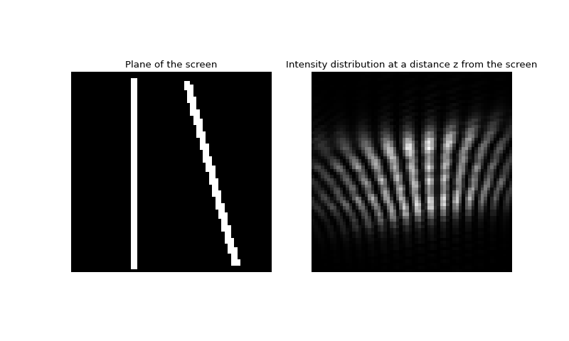
Fig. 10. Intensity distributions in plane of the screen and 75 cm after the screen, note that input and output have different scales, input grid is 2.5x2.5mm, output is 5x5mm.

This example uses approximately 25 times less memory than the previous FFT. The calculation may take long execution time to tens of seconds or more, depending on the speed of the computer.

6.4. Interpolation.

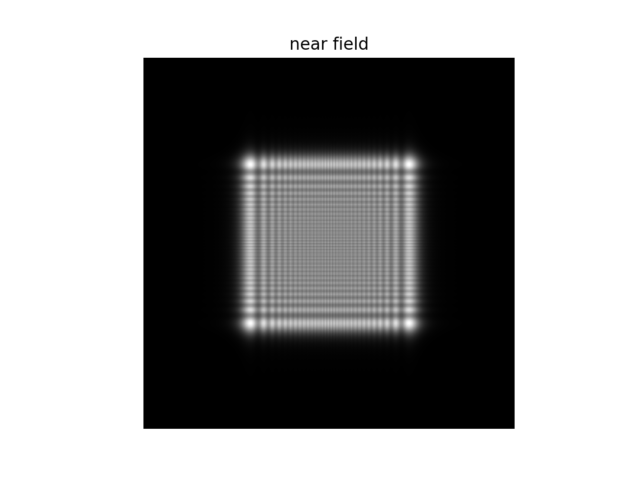
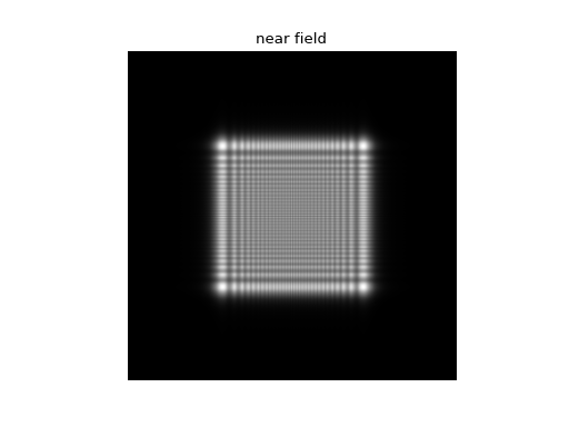
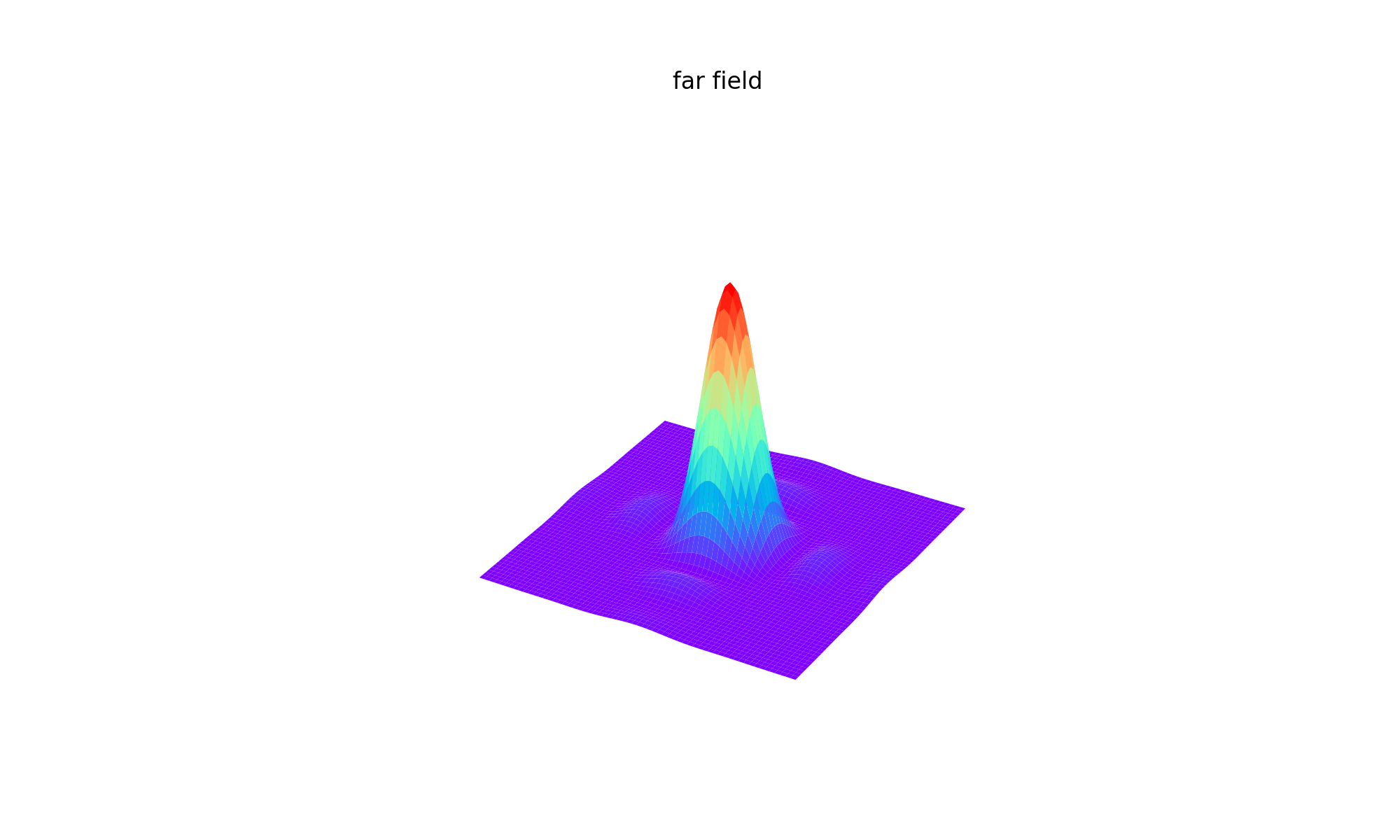
The command Interpol is the tool for manipulating the size and the dimension of the grid and for changing the shift, rotation and the scale of the field distribution. It accepts six command line arguments, the first is the new size of the grid. The second argument gives the new number of points, the third gives the value of transverse shift in the X direction, the fourth gives the shift in the Y direction, the fifth gives the field rotation (first shift and then rotation). The last sixth argument determines the magnification, its action is equivalent to passing the beam through a focal system with magnification M (without diffraction, but preserving the integral intensity). For example if the field was propagated with the FFT algorithm Forvard, then the grid contains empty borders, which is not necessary if we want to propagate the field further with Forward. Other way around, after Forward we have to add some empty borders to continue with Forvard. Interpol is useful for interpolating into a grid with different size and number of points. Of course it is not too wise to interpolate from a grid of 512x512 points into a grid of 8x8, and then back because all information about the field will be lost. The same is true for interpolating the grid of 1mx1m to 1mmx1mm and back. When interpolating into a grid with larger size, for example from 1x1 to 2x2, the program puts zeros into the new added regions. Figure 11 illustrates the usage of Interpol for the transition from a fine grid used by Forvard (near field) to a coarse grid used by Forward (far field).

#! python3

import matplotlib.pyplot as plt
from mpl_toolkits.mplot3d import Axes3D
import numpy as np
from LightPipes import *

print(LPversion)
wavelength=1000*nm
size=10*mm
N=256
w=5*mm

z=400*m
sizenew=400*mm
Nnew=64

F = Begin(size,wavelength,N)

F = RectAperture(w, w,0,0, 0, F)
F = Forvard(0.2*m,F)
I0=Intensity(2,F)

F = Interpol(7.5*mm,Nnew,0,0,0,1,F)
F=Forward(z,sizenew,Nnew,F)
I1=Intensity(2,F)
I1=np.array(I1)
plt.imshow(I0, cmap='gray');plt.axis('off'); plt.title('near field')
plt.show()

(Source code, png, hires.png, pdf)

X=range(Nnew)
Y=range(Nnew)
X, Y=np.meshgrid(X,Y) 
fig=plt.figure(figsize=(10,6))
ax = plt.axes(projection='3d')
ax.plot_surface(X, Y,I1,
                rstride=1,
                cstride=1,
                cmap='rainbow',
                linewidth=0.0,
                )
ax.axis('off'); ax.set_title('far field')
plt.show()

(png, hires.png, pdf)

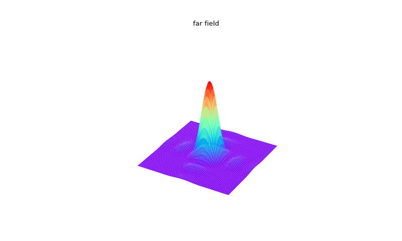
Fig. 11. Illustration of the usage of Interpol for the transition from a fine grid used by Forvard (near field) to a coarse grid used by Forward (far field).

6.5. Phase and intensity filters.

There are four kinds of phase filters available in LightPipes -wave front tilt, the quadratic phase corrector called lens, a general aberration in the form of a Zernike polynomial, and a user defined filter. To illustrate the usage of these filters let’s consider the following examples:

from LightPipes import *
import matplotlib.pyplot as plt

size=40*mm
wavelength=1*um
N=256
w=20*mm
f=8*m
z=4*m

Field = Begin(size, wavelength, N)
Field = RectAperture(w, w, 0, 0, 0, Field)
Field = Lens(f,0,0,Field)
I0 = Intensity(0,Field)
phi0 = Phase(Field)

Field = Forvard(z, Field)
I1 = Intensity(0,Field)

x=[]
for i in range(256):
    x.append((-size/2+i*size/N)/mm)

fig=plt.figure(figsize=(10,6))
ax1 = fig.add_subplot(131)
ax2 = fig.add_subplot(132)
ax3 = fig.add_subplot(133)

ax1.plot(x,phi0[int(N/2)]);ax1.set_xlabel('x [mm]');ax1.set_ylabel('Phase [rad]')
ax2.imshow(I0,cmap='gray'); ax2.axis('off')
ax3.imshow(I1,cmap='gray'); ax3.axis('off')
plt.show()

(Source code, png, hires.png, pdf)

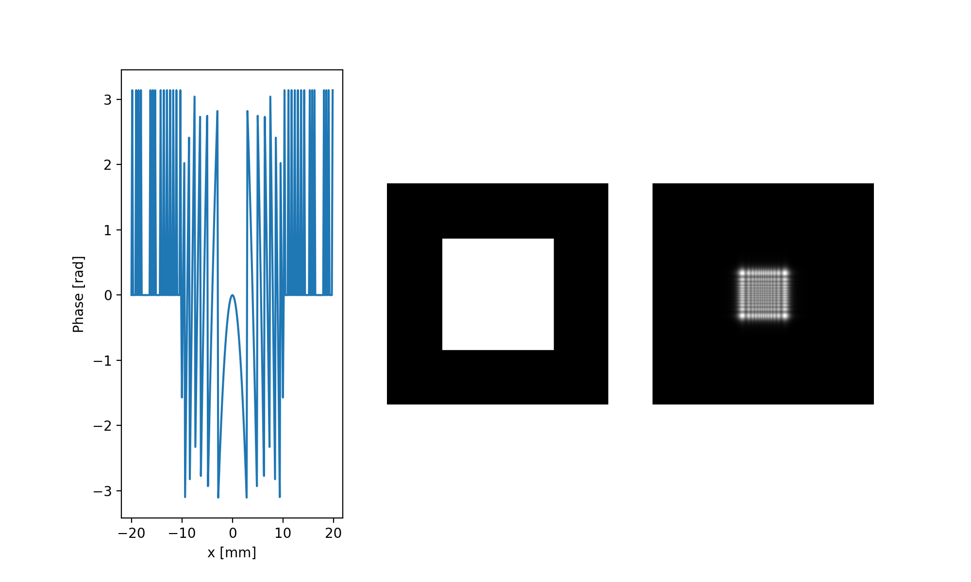
Fig. 12. The phase distribution after passing the lens, intensity in the plane of the lens and at a distance equal to the half of the focal distance. (from left to right)

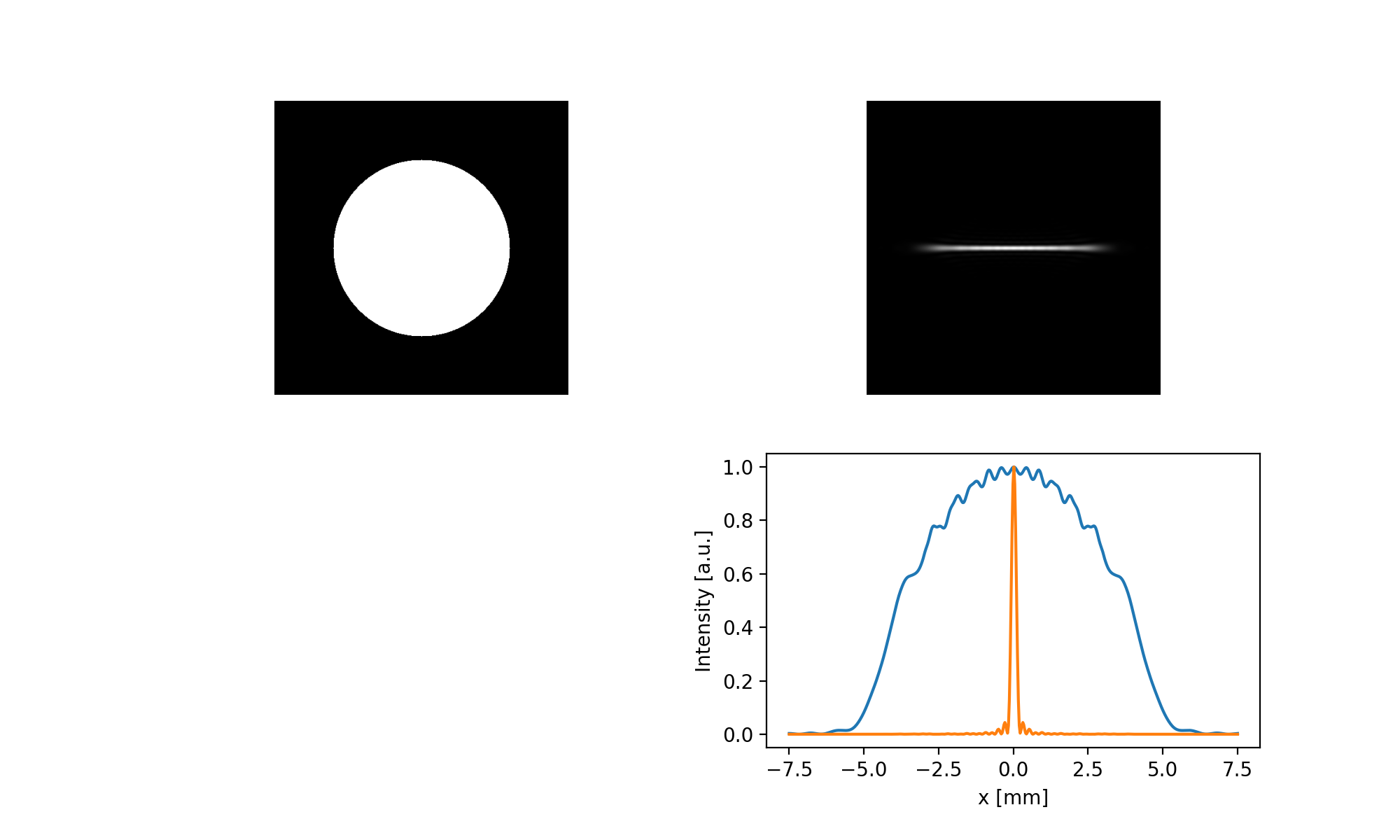
The first sequence of operators forms the initial structure, filters the field through the rectangular aperture and then filters the field through a positive lens with optical power of 0.125D (the focal distance of \(1/0.125=8m\) ). With the second command we propagate the field 4m forward. As 4m is exactly the half of the focal distance, the cross section of the beam must be reduces twice.

We have to be very careful propagating the field to the distance which is close to the focal distance of a positive lens- the near—focal intensity and phase distributions are localised in the central region of the grid occupying only a few grid points. This leads to the major loss of information about the field distribution. The problem is solved by applying the co-ordinate system which is tied to the divergent or convergent light beam, the tools to do this will be described later.

The lens may be decentered, Lens(8, 0.01, 0.01, Field) produces the lens with a focal length of \(1/0.125\) shifted by 0.01 in X and Y directions. Note, when the lens is shifted, the aperture of the lens is not shifted, the light beam is not shifted also, only the phase mask correspondents to the lens is shifted.

The wave front tilt is illustrated by following example:

from LightPipes import *
import matplotlib.pyplot as plt

size=40*mm
wavelength=1*um
N=256
w=20*mm
z=8*m
tx=0.1*mrad
ty=0.1*mrad

Field = Begin(size, wavelength, N)
Field = RectAperture(w, w, 0, 0, 0, Field)
Field = Tilt(tx,ty,Field)
I0 = Intensity(0,Field)


Field = Forvard(z, Field)
I1 = Intensity(0,Field)
phi1 = Phase(Field)

x=[]
for i in range(256):
    x.append((-size/2+i*size/N)/mm)

fig=plt.figure(figsize=(10,6))
ax1 = fig.add_subplot(121)
ax2 = fig.add_subplot(122)


ax1.plot(x,I1[int(N/2)]);ax1.set_xlabel('x [mm]');ax1.set_ylabel('Intensity [a.u.]')
ax2.plot(x,phi1[int(N/2)]);ax2.set_xlabel('x [mm]');ax2.set_ylabel('Phase [rad]')

plt.show()

(Source code, png, hires.png, pdf)

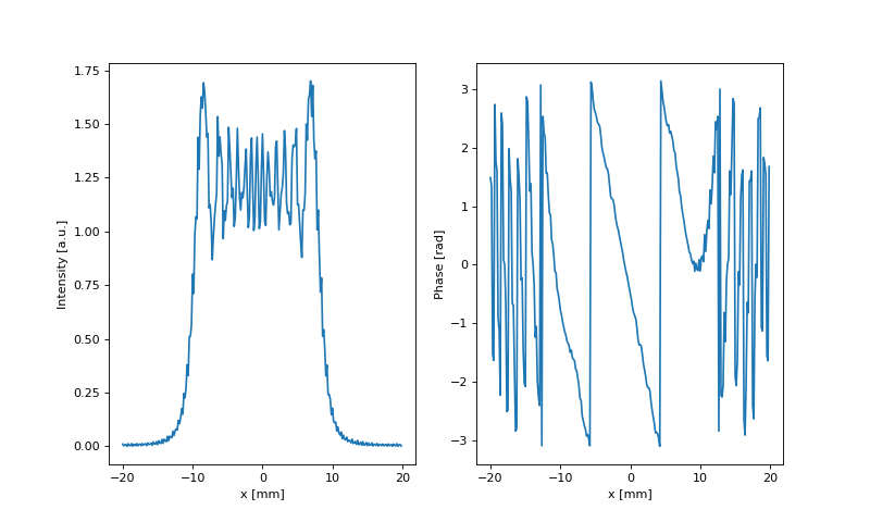
Fig. 13. The intensity and the phase after tilting the wave front by 0.1 mrad and propagating it z = 8 m forward. Note the transversal shift of the intensity distribution and the phase tilt.

In this example the wave front was tilted by \(\alpha = 0.1 mrad\) in X and Y directions, then propagated to the distance \(z = 8 m\) , so in the output distribution we observe the transversal shift of the whole intensity distribution by \(\alpha z = 0.8 mm\) .

6.6. Zernike polynomials.

Any aberration in a circle can be decomposed over a sum of Zernike polynomials. Formulas given in 7 have been directly implemented in LightPipes. The command is called Zernike and accepts four command line arguments:

The radial order n (first column in Table 13.2 8 p. 465).

The azimuthal order \(m\) , \(|m| <= n\) , polynomials with negative \(n\) are rotated \(90^{\circ}\) relative to the polynomials with positive n. For example Zernike(5,3,1,1,Field) gives the same aberration as Zernike(5,-3,1,1,Field), but the last is rotated \(90^{\circ}\) . This index corresponds to the \(n-2m\) given in the third column of Table 13.2 in 8 , p. 465.

The radius, R.

The amplitude of aberration in radians at R.

We can uniformly introduce Lens and Tilt with Zernike, the difference is that we pass the amplitude of the aberration to Lens, Tilt and Zernike accept conventional meters and radians, which are widely in use for the description of optical setups, while Zernike uses the amplitude of the aberration, which frequently has to be derived from the technical description.

A cylindrical lens can be modelled as a combination of two Zernike commands:

from LightPipes import *
import matplotlib.pyplot as plt
import math
import numpy as np
size=15*mm
wavelength=1*um
N=500
R=4.5*mm
z=1.89*m

A = wavelength/(2*math.pi*math.sqrt(2*(2+1)))
Field = Begin(size, wavelength, N)
Field = CircAperture(R, 0, 0, Field)
I0 = Intensity(1,Field)
Field = Zernike(2,2,R,-20*A,Field)
Field = Zernike(2,0,R,10*A,Field)
Field = Fresnel(z, Field)
#Field = Interpol(size,N,0,0,-45,1,Field)
I1 = Intensity(1,Field)
I1=np.array(I1)
x=np.linspace(-size/2.0,size/2.0,N)/mm

fig=plt.figure(figsize=(10,6))
ax1 = fig.add_subplot(221)
ax2 = fig.add_subplot(222)
ax3 = fig.add_subplot(224)

ax1.imshow(I0,cmap='gray'); ax1.axis('off')
ax2.imshow(I1,cmap='gray'); ax2.axis('off')
ax3.plot(x,I1[int(N/2)],x,list(zip(*I1))[int(N/2)])

ax3.set_xlabel('x [mm]');ax3.set_ylabel('Intensity [a.u.]')
plt.show()

(Source code, png, hires.png, pdf)

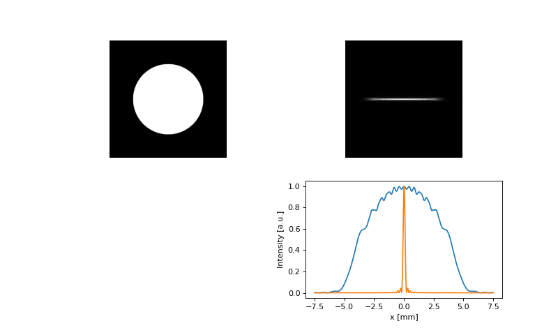
Fig. 14. The intensity in the input plane and after propagation through a cylindrical system modelled as a combination of Zernike polynomials and free space propagation.

6.7. Spherical coordinates.

The principle of beam propagation in the “floating” co-ordinate system (for the case of a lens wave guide) is shown in Figure 15.

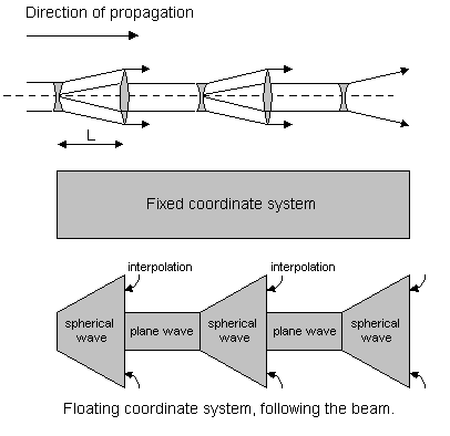
Fig. 15. The intensity in the input plane and after propagation through a cylindrical system modelled as a combination of Zernike polynomials and free space propagation.

The spherical coordinates follow the geometrical section of the divergent or convergent light beam. Propagation in spherical coordinates is implemented with the commands LensForvard and LensFresnel. Both commands accept two parameters: the focal distance of the lens, and the distance of propagation. When LensForvard or LensFresnel is called, it “bends” the coordinate system so, that it follows the divergent or convergent spherical wave front, and then propagates the field to the distance z in the transformed coordinates. The command Convert should be used to convert the field back to the rectangular coordinate system. Some LightPipes commands can not be applied to the field in spherical coordinates. As the coordinates follow the geometrical section of the light beam, operator LensForvard(10,10,Field) will produce floating exception because the calculations can not be conducted in a grid with zero size (that is so in the geometrical approximation of a focal point). On the other hand, diffraction to the focus is equivalent to the diffraction to the far field (infinity), thus the FFT convolution algorithm will not work properly anyway. To model the diffraction into the focal point, a more complicated trick should be used:

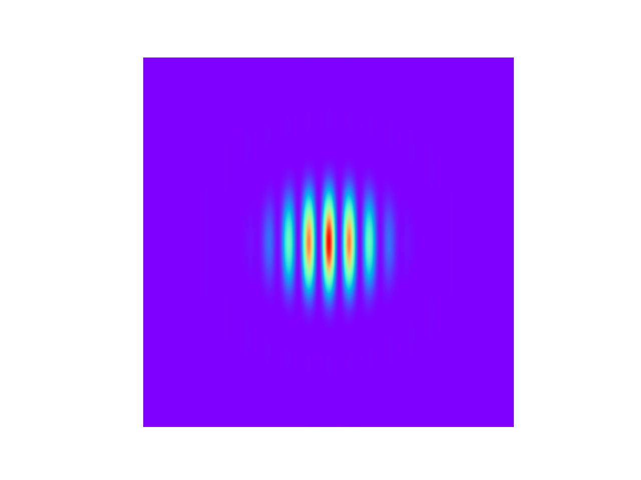
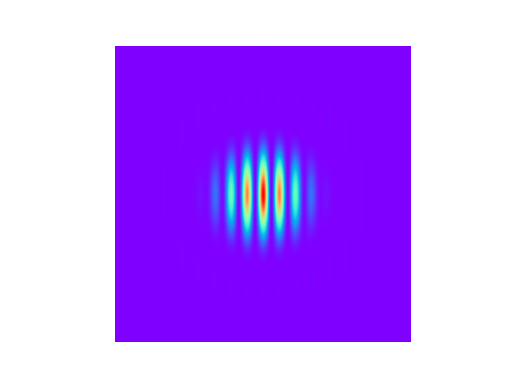
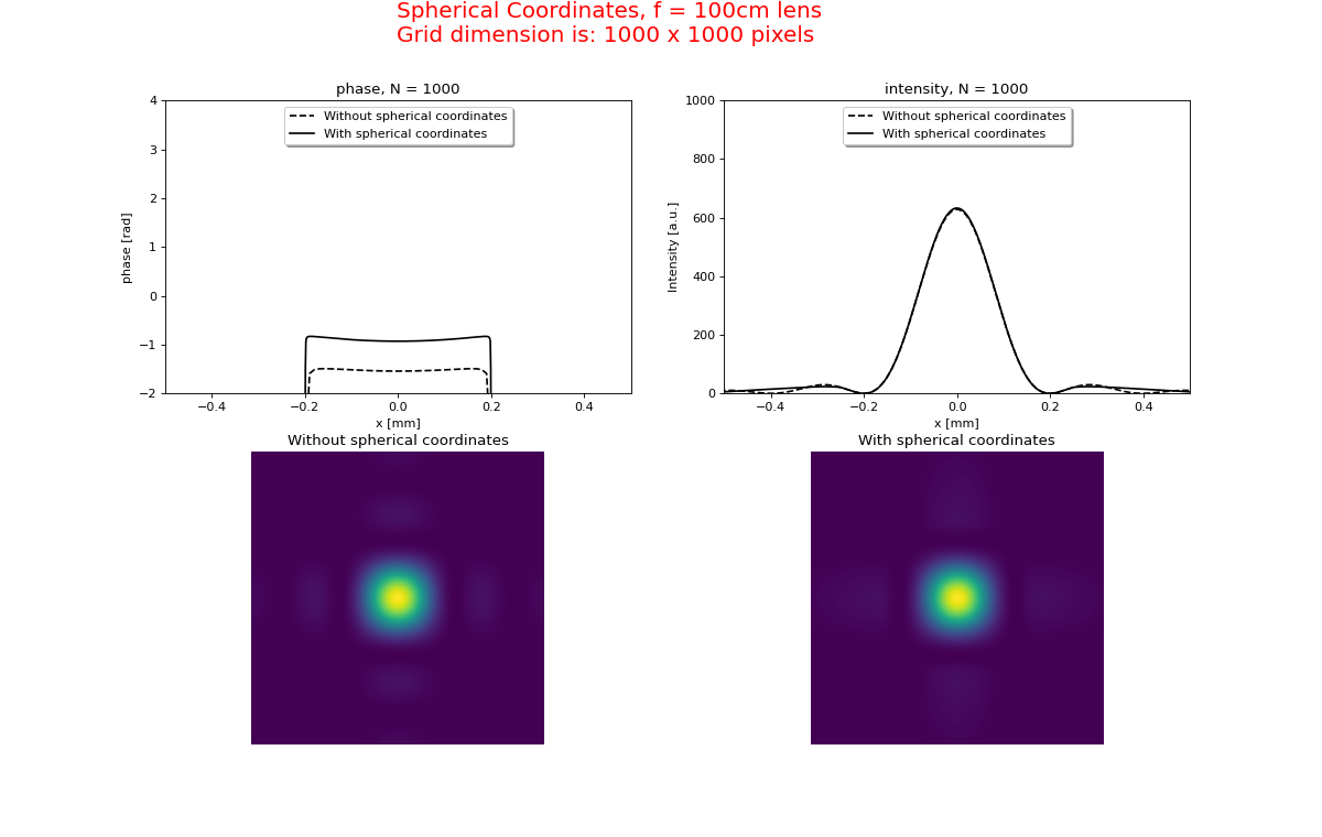
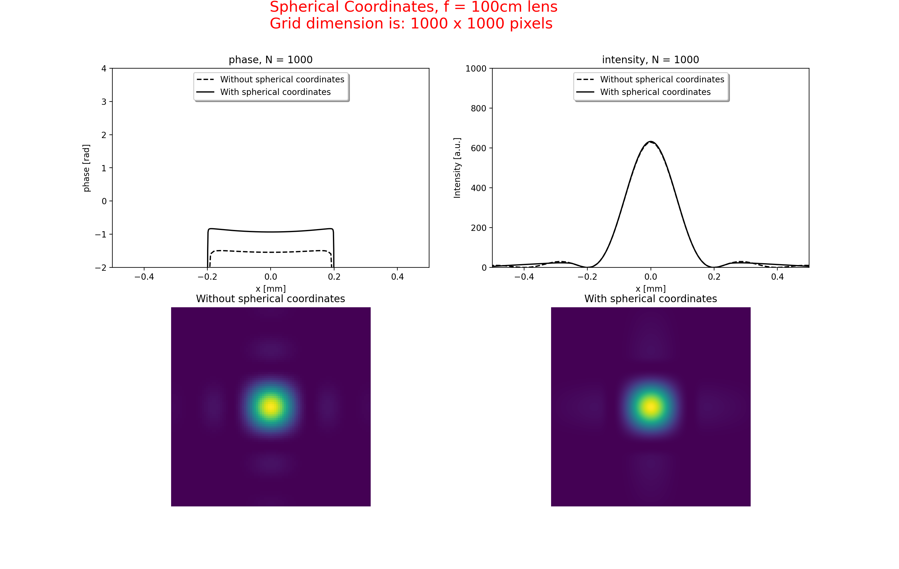
In Figure 16 we calculate the diffraction to the focus of a lens with a focal distance of 1m and compare the spherical coordinate method with the simple straight forward method of a lens followed by propagation to its focus. The spherical coordinates method uses the combination of a weak phase mask Lens(f1, F) and a “strong” geometrical coordinate transform LensFresnel(f2, z, F). The grid after propagation is 10 times narrower than in the input plane. The focal intensity is 650 times higher than the input intensity and the wave front is plain as expected.

The straight-forward method uses the following commands:

labda=1000*nm;
size=10*mm;
f=100*cm
w=5*mm;
F=Begin(size,labda,N);
F=RectAperture(w,w,0,0,0,F);
F1=Lens(f,0,0,F)
F1=Fresnel(f,F1)
phi1=Phase(F1);phi1=PhaseUnwrap(phi1)
I1=Intensity(0,F1);

to calculate the field at the focus of a positive lens.

The method with spherical coordinates is slightly more complex:

labda=1000*nm;
size=10*mm;
f=100*cm
w=5*mm;
f1=10*m
f2=f1*f/(f1-f)
frac=f/f1
newsize=frac*size
F=Begin(size,labda,N);
F=RectAperture(w,w,0,0,0,F);
F2=Lens(f1,0,0,F);
F2=LensFresnel(f2,f,F2);
F2=Convert(F2);
phi2=Phase(F2);phi2=PhaseUnwrap(phi2)
I2=Intensity(0,F2);

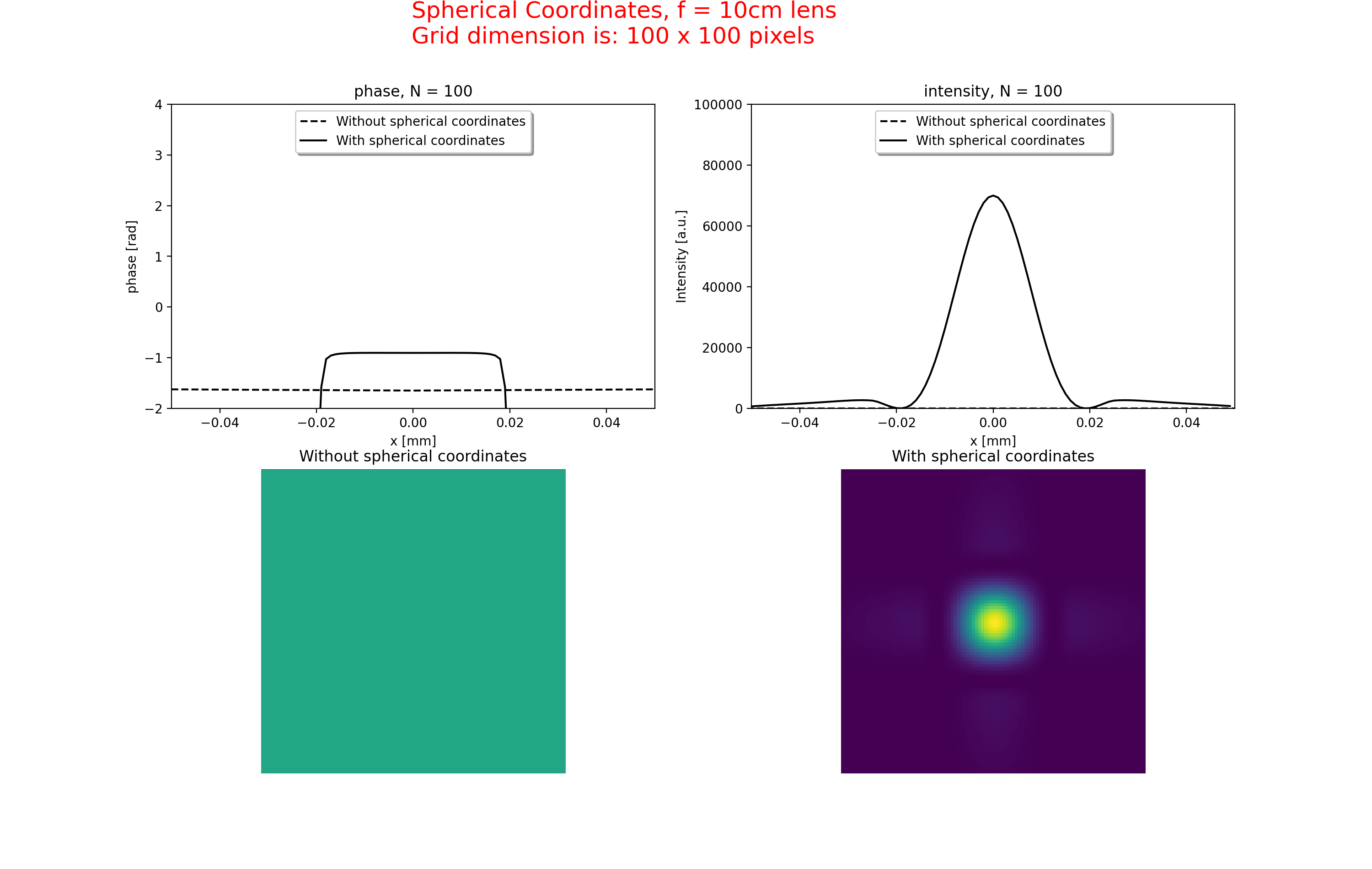
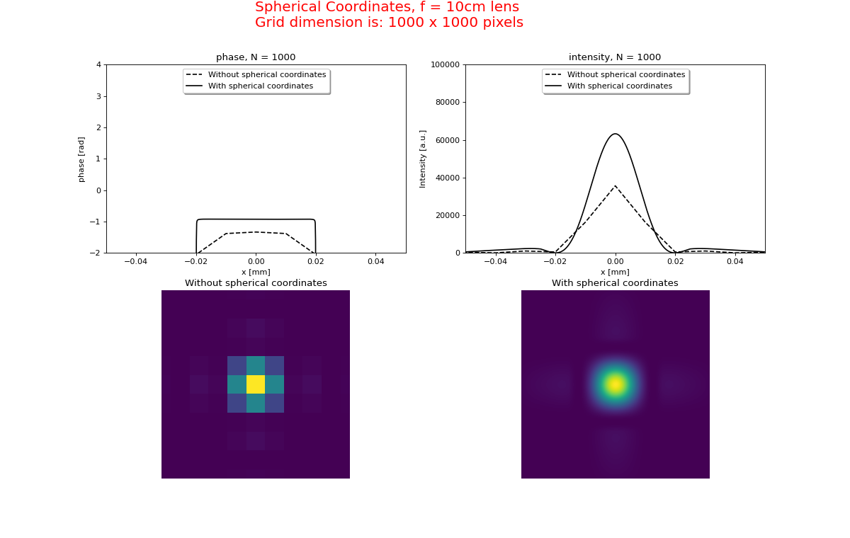
The bending of the coordinate system for the LensFresnel command is given by \(f_2\). The results for \(f=100 cm\) and \(f=10 cm\) are shown in figures 16a+b where the two methods are compared. As can been seen the straight-forward method requires much larger grid dimensions and hence longer execution time. This is especially the case for stronger lenses (shorter focal lengths).

from LightPipes import *
import matplotlib.pyplot as plt

def TheExample(N):
    fig=plt.figure(figsize=(15,9.5))
    ax1 = fig.add_subplot(221)
    ax2 = fig.add_subplot(222)
    ax3 = fig.add_subplot(223)
    ax4 = fig.add_subplot(224)
    labda=1000*nm;
    size=10*mm;

    f=100*cm
    f1=10*m
    f2=f1*f/(f1-f)
    frac=f/f1
    newsize=frac*size
    w=5*mm;
    F=Begin(size,labda,N);
    F=RectAperture(w,w,0,0,0,F);

#1) Using Lens and Fresnel:
    F1=Lens(f,0,0,F)
    F1=Fresnel(f,F1)
    phi1=Phase(F1);phi1=PhaseUnwrap(phi1)
    I1=Intensity(0,F1);
    x1=[]
    for i in range(N):
        x1.append((-size/2+i*size/N)/mm)  

#2) Using Lens + LensFresnel and Convert:
    F2=Lens(f1,0,0,F);
    F2=LensFresnel(f2,f,F2);
    F2=Convert(F2);
    phi2=Phase(F2);phi2=PhaseUnwrap(phi2)
    I2=Intensity(0,F2);
    x2=[]

    for i in range(N):
        x2.append((-newsize/2+i*newsize/N)/mm)

    ax1.plot(x1,phi1[int(N/2)],'k--',label='Without spherical coordinates')
    ax1.plot(x2,phi2[int(N/2)],'k',label='With spherical coordinates');
    ax1.set_xlim(-newsize/2/mm,newsize/2/mm)
    ax1.set_ylim(-2,4)
    ax1.set_xlabel('x [mm]');
    ax1.set_ylabel('phase [rad]');
    ax1.set_title('phase, N = %d' %N)
    legend = ax1.legend(loc='upper center', shadow=True)

    ax2.plot(x1,I1[int(N/2)],'k--',label='Without spherical coordinates')
    ax2.plot(x2,I2[int(N/2)], 'k',label='With spherical coordinates');
    ax2.set_xlim(-newsize/2/mm,newsize/2/mm)
    ax2.set_ylim(0,1000)
    ax2.set_xlabel('x [mm]');
    ax2.set_ylabel('Intensity [a.u.]');
    ax2.set_title('intensity, N = %d' %N)
    legend = ax2.legend(loc='upper center', shadow=True)

    ax3.imshow(I1);ax3.axis('off');ax3.set_title('Without spherical coordinates')
    ax3.set_xlim(int(N/2)-N*frac/2,int(N/2)+N*frac/2)
    ax3.set_ylim(int(N/2)-N*frac/2,int(N/2)+N*frac/2)
    ax4.imshow(I2);ax4.axis('off');ax4.set_title('With spherical coordinates')
    plt.figtext(0.3,0.95,'Spherical Coordinates, f = 100cm lens\nGrid dimension is: %d x %d pixels' %(N, N), fontsize = 18, color='red')

TheExample(100) #100 x 100 grid

TheExample(1000) #1000 x 1000 grid
plt.show()

(Source code)

_images/LensFresnel_Convert_f100cm_00.png — (`png`, `hires.png`, `pdf`)

_images/LensFresnel_Convert_f100cm_01.png — (`png`, `hires.png`, `pdf`)

Fig. 16a. Diffraction to the focus of a f=100 cm lens. The use of a spherical coordinate system (LensFresnel + Convert) is compared with the straight-forward method (Lens + Fresnel).

from LightPipes import *
import matplotlib.pyplot as plt

def TheExample(N):
    fig=plt.figure(figsize=(15,9.5))
    ax1 = fig.add_subplot(221)
    ax2 = fig.add_subplot(222)
    ax3 = fig.add_subplot(223)
    ax4 = fig.add_subplot(224)

    labda=1000*nm;
    size=10*mm;

    f=10*cm
    f1=10*m
    f2=f1*f/(f1-f)
    frac=f/f1
    newsize=frac*size
    w=5*mm;
    F=Begin(size,labda,N);
    F=RectAperture(w,w,0,0,0,F);

#1) Using Lens and Fresnel:
    F1=Lens(f,0,0,F)
    F1=Fresnel(f,F1)
    phi1=Phase(F1);phi1=PhaseUnwrap(phi1)
    I1=Intensity(0,F1);
    x1=[]
    for i in range(N):
        x1.append((-size/2+i*size/N)/mm)  

#2) Using Lens + LensFresnel and Convert:
    F2=Lens(f1,0,0,F);
    F2=LensFresnel(f2,f,F2);
    F2=Convert(F2);
    phi2=Phase(F2);phi2=PhaseUnwrap(phi2)
    I2=Intensity(0,F2);
    x2=[]

    for i in range(N):
        x2.append((-newsize/2+i*newsize/N)/mm)

    ax1.plot(x1,phi1[int(N/2)],'k--',label='Without spherical coordinates')
    ax1.plot(x2,phi2[int(N/2)],'k',label='With spherical coordinates');
    ax1.set_xlim(-newsize/2/mm,newsize/2/mm)
    ax1.set_ylim(-2,4)
    ax1.set_xlabel('x [mm]');
    ax1.set_ylabel('phase [rad]');
    ax1.set_title('phase, N = %d' %N)
    legend = ax1.legend(loc='upper center', shadow=True)

    ax2.plot(x1,I1[int(N/2)],'k--',label='Without spherical coordinates')
    ax2.plot(x2,I2[int(N/2)], 'k',label='With spherical coordinates');
    ax2.set_xlim(-newsize/2/mm,newsize/2/mm)
    ax2.set_ylim(0,100000)
    ax2.set_xlabel('x [mm]');
    ax2.set_ylabel('Intensity [a.u.]');
    ax2.set_title('intensity, N = %d' %N)
    legend = ax2.legend(loc='upper center', shadow=True)

    ax3.imshow(I1);ax3.axis('off');ax3.set_title('Without spherical coordinates')
    ax3.set_xlim(int(N/2)-N*frac/2,int(N/2)+N*frac/2)
    ax3.set_ylim(int(N/2)-N*frac/2,int(N/2)+N*frac/2)
    ax4.imshow(I2);ax4.axis('off');ax4.set_title('With spherical coordinates')
    plt.figtext(0.3,0.95,'Spherical Coordinates, f = 10cm lens\nGrid dimension is: %d x %d pixels' %(N, N), fontsize = 18, color='red')

TheExample(100) #100 x 100 grid

TheExample(1000) #1000 x 1000 grid

plt.show()

(Source code)

_images/LensFresnel_Convert_f10cm_00.png — (`png`, `hires.png`, `pdf`)

_images/LensFresnel_Convert_f10cm_01.png — (`png`, `hires.png`, `pdf`)

Fig 16b. With a stronger lens the straight-forward method requires more grid points.

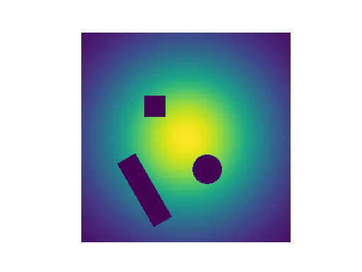
6.8. User defined phase and intensity filters.

The phase and intensity of the light beam can be manipulated in several ways. The phase and intensity distributions may be produced as shown in the next examples:

from LightPipes import *
import matplotlib.pyplot as plt
import math
import numpy as np

size=30*mm
wavelength=1*um
N=256
R=10*mm

Int=np.empty([N,N])
phase=np.empty([N,N])
for i in range(0,N):
    for j in range(0,N):
        Int[i][j]=math.fabs(math.sin(i/10.0)*math.cos(j/5.0))
        phase[i][j]=math.cos(i/10.0)*math.sin(j/5.0)
phase = 0.12345*rad
F=Begin(size,wavelength,N)
F=SubIntensity(F,Int)
F=SubPhase(phase,F)
F=CircAperture(R,0,0,F)

I=Intensity(0,F)
Phi=Phase(F)
fig=plt.figure(figsize=(10,6))
ax1 = fig.add_subplot(121)
ax2 = fig.add_subplot(122)


ax1.imshow(I,cmap='rainbow'); ax1.axis('off'); ax1.set_title('Intensity')
ax2.imshow(Phi,cmap='hot'); ax2.axis('off'); ax2.set_title('Phase')

plt.show()

(Source code, png, hires.png, pdf)

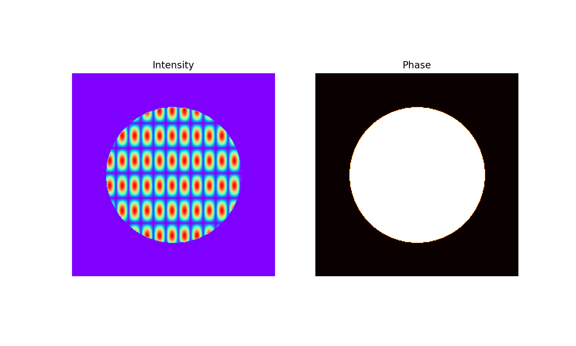
Fig. 17. An arbitrary intensity- and phase distribution.

You can also create your own mask with a program like Microsoft Paint. In the next example we made an arrow using Paint and stored it as a 200 pixels width x 200 pixels height, black-and-white, monochrome bitmap file (for example: arrow.png). This file can be read from disk. Next the arrow can be used as a filter:

from LightPipes import *
import matplotlib.pyplot as plt
import matplotlib.image as mpimg
import math
import numpy as np

#Convert rgb to gray with weighted average of rgb pixels:
def rgb2gray(rgb):
    return np.dot(rgb[...,:3], [0.299, 0.587, 0.114])

#read image from disk and check if it is square:
img=mpimg.imread('arrow.png')
#print(img[100][1])
img=rgb2gray(img)
#print(img[100])
data = np.asarray( img, dtype='uint8' )
Nr=data.shape[0]
Nc=data.shape[1]
if Nc != Nr:
    print ('image must be square')
    exit()
else:
    N=Nc

size=25*mm
wavelength=1*um

R=6*mm
xs=2*mm
ys=0*mm

F=Begin(size,wavelength,N)
F=GaussAperture(R,xs,ys,1,F)
F=MultIntensity(img,F)
I=Intensity(0,F)

plt.imshow(I,cmap='gray'); plt.axis('off'); plt.title('Intensity')
plt.show()

(Source code, png, hires.png, pdf)

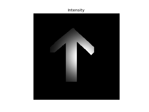
Fig. 18. Illustration of importing a bit map from disk.

6.9. Random filters.

There are two random filters to introduce a random intensity or a random phase distribution in the field. The commands RandomIntensity and RandomPhase need a seed to initiate the random number generator. The RandomPhase command needs a maximum phase value (in radians). The RandomIntensity command yields a normalised random intensity distribution. The RandomIntensity and the RandomPhase commands leave the phase and the intensity unchanged respectively.

6.10. FFT and spatial filters.

LightPipes provide a possibility to perform arbitrary filtering in the Fourier space. There is an operator, performing the Fourier transform of the whole data structure: PipFFT.

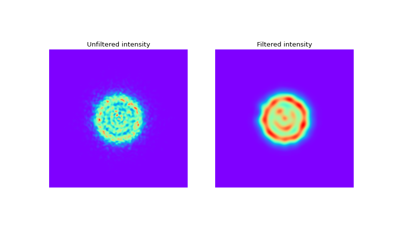
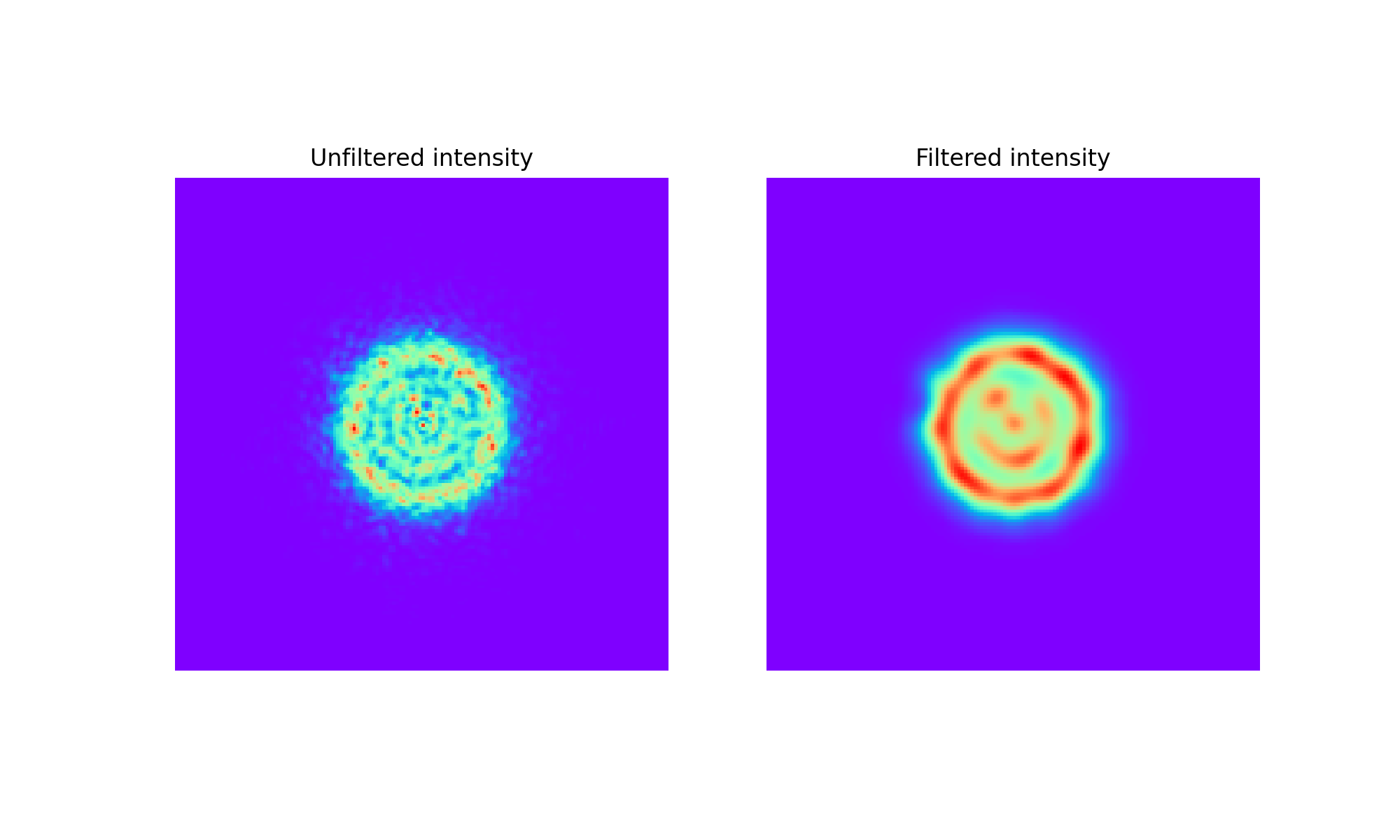
To spatial filter a beam with an aperture the following code could be used:

from LightPipes import *
import matplotlib.pyplot as plt

size=15*mm
wavelength=1*um
N=150
z=1*m
R=3*mm
Rf=1.5*mm
seed=7
MaxPhase=1.5

F=Begin(size,wavelength,N);
F=CircAperture(R,0,0,F);
F=RandomPhase(seed,MaxPhase,F);
F=Fresnel(z,F);
I0=Intensity(0,F);

F=PipFFT(1,F);
F=CircAperture(Rf,0,0,F);
F=PipFFT(-1,F);
I1=Intensity(1,F);

fig=plt.figure(figsize=(10,6))
ax1 = fig.add_subplot(121)
ax2 = fig.add_subplot(122)
ax1.imshow(I0,cmap='rainbow'); ax1.axis('off'); ax1.set_title('Unfiltered intensity')
ax2.imshow(I1,cmap='rainbow'); ax2.axis('off'); ax2.set_title('Filtered intensity')
plt.show()

(Source code, png, hires.png, pdf)

Fig. 19. Intensity distributions before and after applying a spatial filter.

Note, we still can apply all the intensity and phase filters in the Fourier-space. The whole grid size in the angular frequency domain corresponds to \(\frac{2 \pi \lambda}{\Delta x}\), where \(\Delta x\) is the grid step. One step in the frequency domain corresponds to \(\frac{2 \pi \lambda}{x}\), where \(x\) is the total size of the grid. LightPipes filters do not know about all these transformations, so the user should take care about setting the proper size (using the relations mentioned) of the filter (still in linear units) in the frequency domain.

6.11. Laser amplifier.

The Gain command introduces a simple single-layer model of a laser amplifier. The output field is given by: \(F_{out}(x,y) = F_{in}(x,y) e^{\alpha L_{gain}}\), with \(\alpha = \dfrac{\alpha_0}{1 + {2 I(x,y)}/{I_{sat}}}\). \(2\alpha L_{gain}\) is the net round-trip intensity gain. \(\alpha_0\) is the small-signal intensity gain and \(I_{sat}\) is the saturation intensity of the gain medium with a length \(L_{gain}\).

The intensity must be doubled because of the left- and right propagating fields in a normal resonator. (If only one field is propagating in one direction (ring laser) you should double \(I_{sat}\) to remove the factor 2 in the denominator).

The gain sheet should be at one of the mirrors of a (un)stable laser resonator.

6.12. Diagnostics.

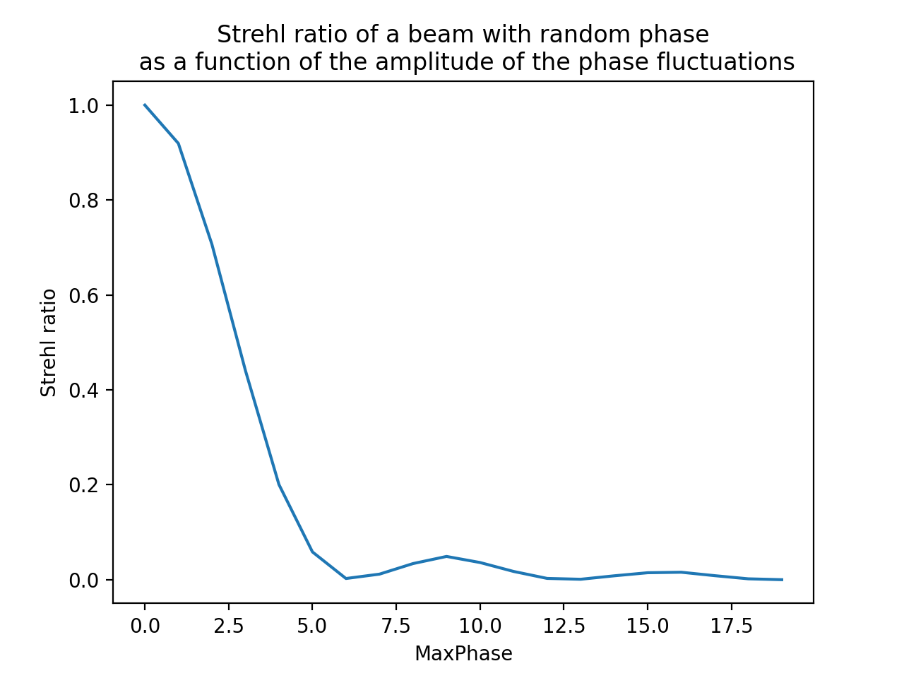
6.12.1. Strehl ratio.

The Strehl command calculates the Strehl ratio of the field, defined as:

\[S= \frac{(\int \int Re(F_{in}(x,y)dxdy)^2 + (\int \int Im(F_{in}(x,y)dxdy)^2}{(\int \int |(F_{in}(x,y)|dxdy)^2}\]

The next example calculates the Strehl ratio of a field with increasing random phase fluctuations:

from LightPipes import *
import matplotlib.pyplot as plt
from mpl_toolkits.mplot3d import Axes3D
import numpy as np
import math

wavelength=1.0*um
size=30*mm
N=200
w=25*mm
S=[]
MaxPhase=[]
for i in range(0,20):
    MaxPhase.append(i)
    seed=i
    F=Begin(size,wavelength,N)
    F=RandomPhase(seed,MaxPhase[i],F)
    S.append(Strehl(F))
plt.plot(MaxPhase,S)
plt.title('Strehl ratio of a beam with random phase\n as a function of the amplitude of the phase fluctuations')
plt.ylabel('Strehl ratio')
plt.xlabel('MaxPhase')
plt.show()

(Source code, png, hires.png, pdf)

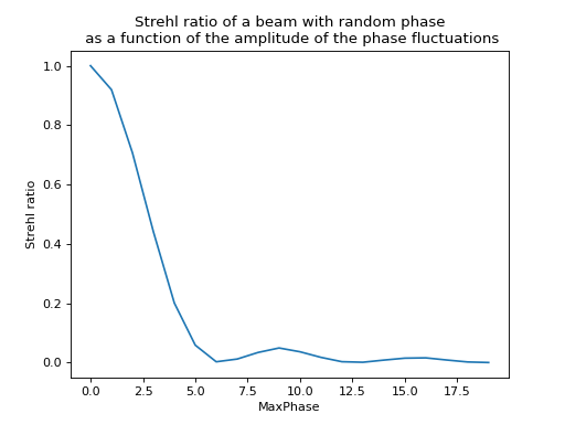
Fig. 21. Demonstration of the use of the Strehl function to calculate the Strehl ratio (beam quality).

6.12.2. Beam power.

The Power command returns the total beam power:

\[P=\int \int(|F_{in}(x,y)|)^2dxdy\]

6.12.3. Field normalization.

The Normal command normalizes the field according to:

\[F_{out}(x,y)=\frac{F_{in}(x,y)}{ \sqrt{P} }\]

\[P=\int \int(|F_{in}(x,y)|)^2dxdy\]

where P is the total beam power.

6.12.4. Centroid.

The Centroid command calculates the centroid of the intensity distribution. It also returns the indices of the Field array closest to the centroid coordinates.

\[X_c=\frac{\int \int xI(x,y)dxdy}{\int \int I(x,y)dxdy}\]

\[Y_c=\frac{\int \int yI(x,y)dxdy}{\int \int I(x,y)dxdy}\]

6.12.5. Beam width.

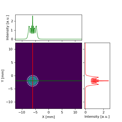
6.12.5.1. \(D4\sigma\)

The D4sigma command returns the width of a beam in the horizontal and vertical direction. It is \(4\) times \(\sigma\), where \(\sigma\) is the standard deviation of the horizontal or vertical marginal distribution respectively. Mathematically, the \(D4\sigma\) beam width in the \(x\) and \(y\) dimension for the beam profile \(I(x,y)\) is expressed as:

\[D4\sigma _x=4\sigma=4\sqrt{\frac{\int \int (x-X_c)^2I(x,y)dxdy}{\int \int I(x,y)dxdy}}\]

\[D4\sigma _y=4\sigma=4\sqrt{\frac{\int \int (y-Y_c)^2I(x,y)dxdy}{\int \int I(x,y)dxdy}}\]

where \(X_c\) and \(Y_c\) are the coordinates of the Centroid.

The next example demonstrates the usage of D4sigma and Centroid:

from LightPipes import *
import matplotlib.pyplot as plt
import numpy as np
from mpl_toolkits.axes_grid1 import make_axes_locatable
from matplotlib import patches

wavelength = 1500*nm
size = 25*mm
N = 500

F=Begin(size,wavelength,N)
F=CircAperture(F, 2*mm, x_shift=-6*mm, y_shift=-2*mm)
F=Fresnel(F, 0.4*m)
Xc,Yc, NXc, NYc =Centroid(F)
sx, sy = D4sigma(F)
I0=Intensity(F)

# Axes ...
fig, main_ax = plt.subplots(figsize=(5, 5))
divider  = make_axes_locatable(main_ax)
top_ax   = divider.append_axes("top",   1.05, pad=0.1, sharex=main_ax)
right_ax = divider.append_axes("right", 1.05, pad=0.1, sharey=main_ax)

# Make some labels invisible
top_ax.xaxis.set_tick_params(labelbottom=False)
right_ax.yaxis.set_tick_params(labelleft=False)

# Labels ...
main_ax.set_xlabel('X [mm]')
main_ax.set_ylabel('Y [mm]')
top_ax.set_ylabel('Intensity [a.u.]')
right_ax.set_xlabel('Intensity [a.u.]')

#plot ...
main_ax.pcolormesh(F.xvalues/mm, F.yvalues/mm, I0)
main_ax.axvline(Xc/mm, color='r')
main_ax.axhline(Yc/mm, color='g')
main_ax.add_patch(patches.Ellipse((Xc/mm, Yc/mm), sx/mm, sy/mm, fill=False, lw=1,color='w', ls='--'))
right_ax.plot(I0[:,NXc],F.yvalues/mm, 'r-', lw=1)
top_ax.plot(F.xvalues/mm,I0[NYc,:], 'g-', lw=1)

plt.show()

(Source code, png, hires.png, pdf)

6.13. References

1(1,2,3)

J.W. Goodman, Introduction to Fourier Optics, 49-56, McGraw-Hill (1968).

2(1,2,3,4)

W.H. Southwell, J. Opt. Soc. Am., 71, 7-14 (1981).

3(1,2,3)

A.E. Siegman, E.A. Sziklas, Mode calculations in unstable resonators with flowing saturable gain: 2. Fast Fourier transform method, Applied Optics 14, 1874-1889 (1975).

4(1,2)

N.N. Elkin, A.P. Napartovich, in “Applied optics of Lasers”, Moscow TsniiAtomInform, 66 (1989) (in Russian).

5

Bacarat, in “The Computer in Optical Research”, ed. B.R. Frieden, Springer Verlag, 72-75 (1980).

6

A.A. Samarskii, E.S. Nikolaev, Numerical Methods for Grid Equations, V.1, Direct methods, pp. 61-65, Birkhäuser Verlag (1989).

7

Born, E. Wolf, Principles of Optics, Pergamon, 464, 767-772 (1993).

8(1,2)

Malacara, Optical shop testing, J. Wiley & Sons, (1992).