4. Command Reference.

ABCD(Fin, M)

Propagates a pure Gaussian field using ABCD matrix theory.

Parameters

Fin (Field) – input field, must be pare Gaussian.
M (List) – 2 x 2 ABCD matrix

Returns

output field (N x N square array of complex numbers).

Return type

LightPipes.field.Field

Example

from LightPipes import *

wavelength = 500*nm
size = 7*mm
N = 1000

w0 = 1*mm
f = 1*m
z = 1*m

M_lens = [
    [1.0,       0.0],
    [-1.0/f,    1.0]
  ]

M_propagate = [
    [1.0,       z ],
    [0.0,       1.0]
  ]

F = Begin(size,wavelength,N)
F = GaussBeam(F, w0,n=0,m=0)
F = ABCD(F,M_lens)
F = ABCD(F,M_propagate)

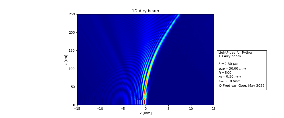
AiryBeam1D(Fin, x0=0.001, a=100)

Creates a 1D nonspreading Airy beam.

\(F(x,y,z=0) = Ai\left(\dfrac{x}{x_0}\right)e^{ax}\)

Parameters

Fin (Field) – input field
x0 (int, float) – scale x (default = 1*mm)
a (int, float) – degree of apodization x (default = 0.1/mm)

Returns

output field (N x N square array of complex numbers).

Return type

LightPipes.field.Field

Example

from LightPipes import *
import matplotlib.pyplot as plt
import numpy as np

wavelength = 2.3*um
size = 30*mm
N = 500
N2=N//2
x0=0.3*mm
a=0.1/mm
dz=1.25*cm
NZ=200

F0=Begin(size,wavelength,N)
F0=AiryBeam1D(F0,x0=x0, a=a)
Ix=np.zeros(N)
for k in range(0,NZ):
    F=Forvard(F0,dz*k)
    I=Intensity(F)
    Ix=np.vstack([Ix,I[N2]])
plt.figure(figsize = (12,5))
plt.imshow(Ix,
           extent=[-size/2/mm, size/2/mm, 0, NZ*dz/cm],
           aspect=0.08,
           origin='lower',
           cmap='jet',
           )
plt.xlabel('x [mm]')
plt.ylabel('z [cm]')
s = r'LightPipes for Python' + '\n'+ '1D Airy beam' + '\n\n'\
    r'$\lambda = {:4.2f}$'.format(wavelength/um) + r' ${\mu}m$' + '\n'\
    r'$size = {:4.2f}$'.format(size/mm) + r' $mm$' + '\n'\
    r'$N = {:4d}$'.format(N) + '\n'\
    r'$x_0 = {:4.2f}$'.format(x0/mm) + r' $mm$' + '\n'\
    r'$a = $' + '{:4.2f}'.format(a*mm) + r' $/mm$' + '\n'\
    r'${\copyright}$ Fred van Goor, May 2022'
plt.text(16, 50, s, bbox={'facecolor': 'white', 'pad': 5})
plt.show()

(Source code, png, hires.png, pdf)

ref: M. V. Berry and N. L. Balazs, “Nonspreading wave packets,” Am. J. Phys. 47, 264–267 (1979).

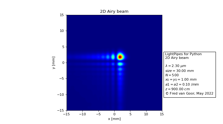
AiryBeam2D(Fin, x0=0.001, y0=0.001, a1=100, a2=100)

Creates a 2D nonspreading Airy beam.

\(F(x,y,z=0) = Ai\left(\dfrac{x}{x_0}\right)Ai\left(\dfrac{y}{y_0}\right)e^{a_1x+a_2y}\)

Parameters

Fin (Field) – input field
x0 (int, float) – scale x (default = 1*mm)
y0 (int, float) – scale y (default = 1*mm)
a1 (int, float) – degree of apodization x (default = 0.1/mm)
a2 (int, float) – degree of apodization y (default = 0.1/mm)

Returns

output field (N x N square array of complex numbers).

Return type

LightPipes.field.Field

Example

from LightPipes import *
import matplotlib.pyplot as plt
import numpy as np

wavelength = 2.3*um
size = 30*mm
N = 500
x0=y0=1*mm
a1=a2=0.1/mm
z=900*cm

F0=Begin(size,wavelength,N)
F0=AiryBeam2D(F0,x0=x0, y0=y0, a1=a1, a2=a2)
F=Fresnel(F0,z)
I=Intensity(F)
plt.figure(figsize = (9,5))
plt.imshow(I,
           extent=[-size/2/mm, size/2/mm, -size/2/mm, size/2/mm],
           origin='lower',
           cmap='jet',
           )
plt.title('2D Airy beam')
plt.xlabel('x [mm]')
plt.ylabel('y [mm]')
s = r'LightPipes for Python' + '\n'+ '2D Airy beam' + '\n\n'\
    r'$\lambda = {:4.2f}$'.format(wavelength/um) + r' ${\mu}m$' + '\n'\
    r'$size = {:4.2f}$'.format(size/mm) + r' $mm$' + '\n'\
    r'$N = {:4d}$'.format(N) + '\n'\
    r'$x_0 = y_0 = {:4.2f}$'.format(x0/mm) + r' $mm$' + '\n'\
    r'$a1 = a2 =  $' + '{:4.2f}'.format(a1*mm) + r' $/mm$' + '\n'\
    r'$z = $' + '{:4.2f}'.format(z/cm) + r' $cm$' + '\n'\
    r'${\copyright}$ Fred van Goor, May 2022'
plt.text(16, -10, s, bbox={'facecolor': 'white', 'pad': 5})
plt.show()

(Source code, png, hires.png, pdf)

ref: M. V. Berry and N. L. Balazs, “Nonspreading wave packets,” Am. J. Phys. 47, 264–267 (1979).

See also

Examples: Non-diffracting Airy beams

Axicon(Fin, phi, n1=1.5, x_shift=0.0, y_shift=0.0)

Propagates the field through an axicon.

Parameters

Fin (Field) – input field
phi (int, float) – top angle of the axicon in radiants
n1 – refractive index of the axicon material (default = 1.5)
x_shift (int, float) – shift in x direction (default = 0.0)
y_shift (int, float) – shift in y direction (default = 0.0)

Returns

output field (N x N square array of complex numbers).

Return type

LightPipes.field.Field

Example

>>> phi=179.7/180*3.1415
>>> F = Axicon(F, phi) # axicon with top angle phi, refractive index = 1.5, centered in grid
>>> F = Axicon(F,phi, n1 = 1.23, y_shift = 2*mm) # Idem, refractive index = 1.23, shifted 2 mm in y direction
>>> F = Axicon(F, phi, 1.23, 2*mm, 0.0) # Idem

See also

Example: Bessel beam with axicon

BeamMix(Fin1, Fin2)

Addition of the fields Fin1 and Fin2.

Parameters

Fin1 (Field) – First field.
Fin2 – Second field
Fin2 – Field

Returns

output field (N x N square array of complex numbers).

Return type

LightPipes.field.Field

Example

>>> F = BeamMix(F1 , F2)

See also

Begin(size, labda, N, dtype=None)

Initiates a field with a grid size, a wavelength and a grid dimension. By setting dtype to numpy.complex64 memory can be saved. If dtype is not set (default = None), complex (equivalent to numpy.complex128) will be used for the field array.

Parameters

size (int, float) – size of the square grid
labda (int, float) – the wavelength of the output field
N (int) – the grid dimension
dtype (complex, numpy.complex64, numpy.complex128 (default = None)) – type of the field array

Returns

output field (N x N square array of complex numbers).

Return type

LightPipes.field.Field

Example

>>> from LightPipes import *
>>> size = 20*mm
>>> wavelength = 500*nm
>>> N = 5
>>> F = Begin(size, wavelength, N)
>>> F
<LightPipes.field.Field object at 0x0000027AAF6E5908>
>>> F.field
array([[1.+0.j, 1.+0.j, 1.+0.j, 1.+0.j, 1.+0.j],
       [1.+0.j, 1.+0.j, 1.+0.j, 1.+0.j, 1.+0.j],
       [1.+0.j, 1.+0.j, 1.+0.j, 1.+0.j, 1.+0.j],
       [1.+0.j, 1.+0.j, 1.+0.j, 1.+0.j, 1.+0.j],
       [1.+0.j, 1.+0.j, 1.+0.j, 1.+0.j, 1.+0.j]])
>>> F.siz
0.02
>>> F.lam
5.000000000000001e-07
>>> F.N
5

See also

Centroid(Fin)

Returns the centroid of the intensity distribution.

Parameters: Fin (Field) – input field.
Returns: the coordinates and the closests array indices of the centroid: Xc, Yc, NXc, NYc
Return type: Tuple[float, float, int, int]
Example

from LightPipes import *
wavelength = 500*nm
size = 25*mm
N = 500
F = Begin(size, wavelength, N)
F = CircAperture(F, 2*mm, x_shift = 5*mm, y_shift = 3*mm)
F = Fresnel(F, 10*m)
Xc,Yc, NXc, NYc = Centroid(F)
print("Xc = {:4.2f} mm, Yc = {:4.2f} mm".format(Xc/mm, Yc/mm))

Answer

Xc = 4.96 mm, Yc = 2.97 mm
NXc =  349, NYc =  309

See also

Manual: Diagnostics: Centroid.

CircAperture(Fin, R, x_shift=0.0, y_shift=0.0)

Inserts a circular aperture in the field.

Parameters

R (int, float) – radius of the aperture
x_shift (int, float) – shift in x direction (default = 0.0)
y_shift (int, float) – shift in y direction (default = 0.0)
Fin (Field) – input field

Returns

output field (N x N square array of complex numbers).

Return type

LightPipes.field.Field

Example

>>> F = CircAperture(F, 3*mm) # A 3 mm radius circular aperture in the center of the grid.
>>> # alternative notations:
>>> F = CircAperture(F, 3*mm, 0, -3*mm) # Shifted -3 mm in the y-direction.
>>> F = CircAperture(F, R = 3*mm, y_shift = -3*mm) # Idem
>>> F = CircAperture(3*mm, 0.0, -3*mm, F) # Idem, old order of arguments for backward compatibility.

See also

CircScreen(Fin, R, x_shift=0.0, y_shift=0.0)

Inserts a circular screen in the field.

Parameters

Fin (Field) – input field
R (int, float) – radius of the screen
x_shift (int, float) – shift in x direction (default = 0.0)
y_shift (int, float) – shift in y direction (default = 0.0)

Returns

output field (N x N square array of complex numbers).

Return type

LightPipes.field.Field

Example

>>> F = CircScreen(F, 3*mm) # A 3 mm radius circular screen in the center of the grid.
>>> # alternative notations:
>>> F = CircScreen(F, 3*mm, 0, -3*mm) # Shifted -3 mm in the y-direction.
>>> F = CircScreen(F, R = 3*mm, y_shift = -3*mm) # Idem
>>> F = CircScreen(3*mm, 0.0, -3*mm, F) # Idem, old order of arguments for backward compatibility.

See also

Convert(Fin)

Converts the field from a spherical variable coordinate to a normal coordinate system.

Parameters: Fin (Field) – input field
Returns: output field (N x N square array of complex numbers).
Return type: LightPipes.field.Field
Example

>>> F = Convert(F) # convert to normal coordinates

See also

Examples: Unstable resonator

CylindricalLens(Fin, f, x_shift=0.0, y_shift=0.0, angle=0.0)

Inserts a cylindrical lens in the field

Parameters

Fin (Field) – input field
f (int, float) – focal length
x_shift (int, float) – shift in the x-direction (default = 0.0)
y_shift (int, float) – shift in the y-direction (default = 0.0)
angle (int, float) – rotation angle (default = 0.0, horizontal)

Returns

output field (N x N square array of complex numbers).

Return type

LightPipes.field.Field

Example

>>> F=Begin(size,wavelength,N)
>>> F=CylindricalLens(F,f) #Cylindrical lens in the center
>>> F=CylindricalLens(F,f, x_shift=2*mm) #idem, shifted 2 mm in x direction
>>> F=CylindricalLens(F,f, x_shift=2*mm, angle=30.0*deg) #idem, rotated 30 degrees

See also

Examples: Transformation of high order Gauss modes

D4sigma(Fin)

Returns the width ( \(D4\sigma\) ) of the intensity distribution.

Parameters: Fin (Field) – input field.
Returns: widths in X and Y direction.
Return type: Tuple[float, float]
Example

from LightPipes import *
wavelength = 500*nm
size = 25*mm
N = 500
F = Begin(size, wavelength, N)
F = CircAperture(F, 2*mm, x_shift = 5*mm, y_shift = 3*mm)
F = Fresnel(F, 10*m)
sx, sy = D4sigma(F)
print("sx = {:4.2f} mm, sy = {:4.2f} mm".format(sx/mm, sy/mm))

Answer

sx = 6.19 mm, sy = 6.30 mm

See also

Manual => Diagnostics => Beam width => D4sigma

FieldArray2D(Fin, Ffield, Nfieldsx, Nfieldsy, x_sep, y_sep)

Inserts an array of fields in the field

Parameters

Fin (Field) – input field
Ffield (Field) – field to be inserted
Nfieldsx (int, float) – number of inserted field in x-direction
Nfieldy (int, float) – number of inserted field in y-direction
x_sep (int, float) – separation of the inserted fields in the x-direction
y_sep (int, float) – separation of the inserted fields in the y-direction

Returns

output field (N x N square array of complex numbers).

Return type

LightPipes.field.Field

Example

>>> #Insert an array of lenses in the field    
>>> F=Begin(size,wavelength,N)
>>> #Define the field, Ffield, to be inserted:
>>> Nfield=int(size_field/size*N)
>>> Ffield=Begin(size_field,wavelength,Nfield)
>>> Ffield=CircAperture(Ffield,Dlens/2)
>>> Ffield=Lens(Ffield,f)
>>> #Insert the Ffield's in the field F:
>>> F=FieldArray2D(F,Ffield,Nfields,Nfields,x_sep,y_sep)
>>> Ifields=Intensity(F)

See also

Examples: Shack Hartmann sensor

Forvard(Fin, z, usepyFFTW=False)

Propagates the field using a FFT algorithm.

Parameters

Fin (Field) – input field
z (int, float) – propagation distance
usepyFFTW (bool) – use the pyFFTW Fast Fourier package (default = False) Has no effect if _USEPYFFTW = True in config.py

Returns

output field (N x N square array of complex numbers).

Return type

LightPipes.field.Field

Examples

>>> F = Forvard(F, 20*cm) # propagates the field 20 cm
>>> F = Forvard(F, 20*cm, usepyFFTW = True) # propagates the field 20 cm using the pyFFTW package
>>> F = Forvard(F, 20*cm, usepyFFTW = False) # propagates the field 20 cm using numpy FFT

See also

Forward(Fin, z, sizenew, Nnew)

Propagates the field using direct integration.

Parameters

Fin (Field) – input field
z (int, float) – propagation distance

Returns

output field (N x N square array of complex numbers).

Return type

LightPipes.field.Field

Example

>>> F = Forward(F, 20*cm, 10*mm, 20) # propagates the field 20 cm, for a new grid size of 10 mm and a new grid dimension 20

See also

Manual: Direct integration.
Manual: Splitting and mixing beams. (figure 10.)

Fresnel(Fin, z, usepyFFTW=False)

Propagates the field using a convolution method.

Parameters

Fin (Field) – input field
z (int, float) – propagation distance
usepyFFTW (bool) – use the pyFFTW Fast Fourier package (default = False) Has no effect if _USEPYFFTW = True in config.py

Returns

output field (N x N square array of complex numbers).

Return type

LightPipes.field.Field

Examples

>>> F = Fresnel(F, 20*cm) # propagates the field 20 cm
>>> F = Fresnel(F, 20*cm, usepyFFTW = True) # propagates the field 20 cm using the pyFFTW package
>>> F = Fresnel(F, 20*cm, usepyFFTW = False) # propagates the field 20 cm using numpy fft

See also

GForvard(Fin, z)

Propagates a pure Gaussian field using ABCD matrix theory.

Parameters

Fin (Field) – input field, must be pare Gaussian.
z (int, float) – propagation distance

Returns

output field (N x N square array of complex numbers).

Return type

LightPipes.field.Field

Example

from LightPipes import *

wavelength = 500*nm
size = 7*mm
N = 1000

w0 = 1*mm
z = 1*m

F = Begin(size,wavelength,N)
F = GaussBeam(F, w0,n=0,m=0)
F = GForvard(F,z)      

GLens(Fin, f)

Propagates the field through an ideal thin lens using ABCD matrix theory. Only works for a pure Gaussian input field.

Parameters

Fin (Field) – input field (must be pure Gaussian)
f (int, float) – focal length of the lens

Returns

output field (N x N square array of complex numbers, pure Gauss).

Return type

LightPipes.field.Field

Example

>>> F = GLens(F,f)

See also

Manual: Phase and intensity filters.

Gain(Fin, Isat, alpha0, Lgain)

Propagates the field through a thin saturable gain sheet.

\(F_{out}(x,y) = F_{in}(x,y) e^{\alpha L_{gain}}\), with \(\alpha = \dfrac{\alpha_0}{1 + {2 I(x,y)}/{I_{sat}}}\).

\(2\alpha L_{gain}\) is the net round-trip intensity gain. \(\alpha_0\) is the small-signal intensity gain and \(I_{sat}\) is the saturation intensity of the gain medium with a length \(L_{gain}\).

The intensity must be doubled because of the left- and right propagating fields in a normal resonator. (If only one field is propagating in one direction (ring laser) you should double \(I_{sat}\) as well to remove the factor 2 in the denominator).

The gain sheet should be at one of the mirrors of a (un)stable laser resonator.

See: Rensch and Chester (1973).

Parameters

Fin (Field) – input field
Isat (int, float) – saturation intensity
alpha0 (int, float) – small signal gain
Lgain (int, float) – length of the gain medium

Returns

output field (N x N square array of complex numbers).

Return type

LightPipes.field.Field

Example

>>> Isat=131*W/cm/cm; alpha=0.0067/cm; Lgain=30*cm;
>>> F = Gain(F, Isat, alpha, Lgain) # amplifacation of the field

See also

Examples: Unstable laser resonator

GaussAperture(Fin, w, x_shift=0.0, y_shift=0.0, T=1.0)

Inserts an aperture with a Gaussian shape in the field.

\(F_{out}(x,y)= \sqrt{T}e^{ -\frac{ x^{2}+y^{2} }{2w^{2}} } F_{in}(x,y)\)

Parameters

Fin (Field) – input field
w (int, float) – 1/e intensity width
x_shift (int, float) – shift in x direction (default = 0.0)
y_shift (int, float) – shift in y direction (default = 0.0)
T (int, float) – center intensity transmission (default = 1.0)

Returns

output field (N x N square array of complex numbers).

Return type

LightPipes.field.Field

Example

>>> F = GaussAperture(Fin, w) # centered, T=1.0, width = w
>>> F = GaussAperture(Fin, w, T = 0.5) # idem, transmission = 0.5
>>> F = GaussAperture(Fin, w, T = 0.5, y_shift = -3 *mm) # idem, shifted in y direction
>>> F = GaussAperture(Fin, w, 0.0, -3.0*mm, 0.5) # idem

See also

Manual: Apertures and screens.

GaussBeam(Fin, w0, n=0, m=0, x_shift=0, y_shift=0, tx=0, ty=0, doughnut=False, LG=False)

Creates a Gaussian beam in its waist.

Parameters

Fin (Field) – input field
w0 – size of the Gauss waist
x_shift (int, float) – shift in x direction (default = 0.0)
y_shift (int, float) – shift in y direction (default = 0.0)
tx (int, float) – tilt in radiants (default = 0.0)
ty (int, float) – tilt in radiants (default = 0.0)
doughnut (bool) – if True a dougnut mode is generated (default = False)
LG (bool) – if True a (n,m) Laguerre-Gauss mode is generated, if False a Hermite Gauss mode (default = False)

Returns

output field (N x N square array of complex numbers).

Return type

LightPipes.field.Field

Example

>>> w0 = 3*mm
>>> F=GaussBeam(w0,F) #TEM0,0 Hermite Gauss beam with size (radius) 3 mm in center of the grid
>>> F=GaussBeam(w0,F,LG=True,n=2,m=5) # LG2,5 Laguerre Gauss beam
>>> F=GaussBeam(w0,F,doughnut=True,m=1) # LG0,1* doughnut beam
>>> F=GaussBeam(w0,F,doughnut=True,m=1, tx = 1*mrad, x_shift = 1*mm) #  idem, tilted and shifted

GaussHermite(Fin, w0, m=0, n=0, A=1.0)

Substitutes a Hermite-Gauss mode (beam waist) in the field.

\(F_{m,n}(x,y,z=0) = A H_m\left(\dfrac{\sqrt{2}x}{w_0}\right)H_n\left(\dfrac{\sqrt{2}y}{w_0}\right)e^{-\frac{x^2+y^2}{w_0^2}}\)

Parameters

Fin (Field) – input field
w0 (int, float) – Gaussian spot size parameter in the beam waist (1/e amplitude point)
m (int, float) – mode index (default = 0.0)
n (int, float) – mode index (default = 0.0)
A (int, float) – amplitude (default = 1.0)

Returns

output field (N x N square array of complex numbers).

Return type

LightPipes.field.Field

Example

>>> F = GaussHermite(F, 3*mm) # Fundamental Gauss mode, HG0,0 with a beam radius of 3 mm
>>> F = GaussHermite(F, 3*mm, m=3) # Idem, HG3,0
>>> F = GaussHermite(F, 3*mm, m=3, n=1, A=2.0) # Idem, HG3,1, amplitude 2.0
>>> F = GaussHermite(F, 3*mm, 3, 1, 2.0) # Idem

See also

Examples: Hermite Gauss modes.

Reference:

A. Siegman, "Lasers", p. 642

GaussLaguerre(Fin, w0, p=0, l=0, A=1.0, ecs=1)

Substitutes a Laguerre-Gauss mode (beam waist) in the field.

\(F_{p,l}(x,y,z=0) = A \left(\rho\right)^{\frac{|l|}{2} }L^p_l(\rho)e^{-\frac{\rho}{2}}\cos(l\theta)\),

with: \(\rho=\frac{2(x^2+y^2)}{w_0^2}\)

\(\theta=atan(y/x)\)

if \(sincos = 0\) replace \(cos(l\theta)\) by \(exp(-il\theta)\)

if \(sincos = 2\) replace \(cos(l\theta)\) by \(sin(l\theta)\)

Parameters

Fin (Field) – input field
w0 (int, float) – Gaussian spot size parameter in the beam waist (1/e amplitude point)
p (int, float) – mode index (default = 0.0)
l (int, float) – mode index (default = 0.0)
A (int, float) – amplitude (default = 1.0)
ecs (int, float) – 0 = exp, 1 = cos, 2 = sin (default = 1)

Returns

output field (N x N square array of complex numbers).

Return type

LightPipes.field.Field

Example

>>> F = GaussLaguerre(F, 3*mm) # Fundamental Gauss mode, LG0,0 with a beam radius of 3 mm
>>> F = GaussLaguerre(F, 3*mm, p=3) # Idem, LG3,0
>>> F = GaussLaguerre(F, 3*mm, p=3, l=1, A=2.0) # Idem, LG3,1, amplitude 2.0
>>> F = GaussLaguerre(F, 3*mm, 3, 1, 2.0) # Idem
>>> F = GaussLaguerre(F, 3*mm, p=3, l=2, ecs=0) LG3,1 with exponential phase factor
>>> F = GaussLaguerre(F, 3*mm, p=3, l=2, ecs=2) LG3,1 with sine phase factor

See also

Examples: Laguerre Gauss modes.

Reference:

A. Siegman, "Lasers", p. 642

GaussScreen(Fin, w, x_shift=0.0, y_shift=0.0, T=0.0)

Inserts a screen with a Gaussian shape in the field.

\(F_{out}(x,y)= \sqrt{1-(1-T)e^{ -\frac{ x^{2}+y^{2} }{w^{2}} }} F_{in}(x,y)\)

Parameters

Fin (Field) – input field
w (int, float) – 1/e intensity width
x_shift (int, float) – shift in x direction (default = 0.0)
y_shift (int, float) – shift in y direction (default = 0.0)
T (int, float) – center intensity transmission (default = 0.0)

Returns

output field (N x N square array of complex numbers).

Return type

LightPipes.field.Field

Example

>>> F = GaussAperture(Fin, w) # centered, T=1.0, width = w
>>> F = GaussAperture(Fin, w, T = 0.5) # idem, transmission = 0.5
>>> F = GaussAperture(Fin, w, T = 0.5, y_shift = -3 *mm) # idem, shifted in y direction
>>> F = GaussAperture(Fin, w, 0.0, -3.0*mm, 0.5) # idem

See also

Manual: Apertures and screens.

IntAttenuator(Fin, att=0.5)

Attenuates the intensity of the field.

\(F_{out}(x,y)=\sqrt{att}F_{in}(x,y)\)

Parameters

Fin (Field) – input field
att (int, float) – intensity attenuation factor (default = 0.5)

Returns

output field (N x N square array of complex numbers).

Return type

LightPipes.field.Field

Example

>>> F = IntAttenuator(F) # attenuates the intensity of the field with a factor 0.5
>>> F = IntAttenuator(F, att = 0.2) # Idem, with a factor 0.2
>>> F = IntAttenuator(F, 0.2) # Idem

See also

Intensity(Fin, flag=0)

Calculates the intensity of the field.

\(I(x,y)=F_{in}(x,y).F_{in}(x,y)^*\)

Parameters

Fin (Field) – input field
flag (int, float) – 0: no normalisation, 1: normalisation to 1, 2: normalized to 255 (for bitmaps) (default = 0)

Returns

output intensity distribution (N x N square array of real numbers).

Return type

numpy.ndarray

Example

>>> I = Intensity(F) # intensity of the field, no normalisation
>>> I = Intensity(F, flag=1) # Idem, normalized to 1
>>> I = Intensity(F, 2) # Idem, normalized to 255

See also

Manual: Graphing and visualisation.

Interpol(Fin, new_size, new_N, x_shift=0.0, y_shift=0.0, angle=0.0, magnif=1.0)

Interpolates the field to a new grid size, grid dimension.

Parameters

Fin (Field) – input field
new_size (int, float) – new grid size
new_N (int, float) – new grid dimension
x_shift (int, float) – shift of the field in x direction (default = 0.0)
y_shift (int, float) – shift of the field in y direction (default = 0.0)
angle (int, float) – rotation of the field in degrees (default = 0.0)
magnif – magnification of the field amplitude (default = 1.0)

Returns

output field (N x N square array of complex numbers).

Return type

LightPipes.field.Field

Example

>>> F = Interpol(F, 50*mm, 200) # interpolates the field to a grid size of 50 mm and a grid dimension of 200
>>> F = Interpol(F, 50*mm, 200, y_shift = 2*mm) # Idem, shifted 2 mm in the y direction
>>> F = Interpol(F, 50*mm, 200, y_shift = 2*mm, magnif = 2.0) # Idem, magnifizes the field a factor 2.0
>>> F = Interpol(F, 50*mm, 200, 0.0, 2*mm, 0.0, 2.0) # Idem

See also

Manual: Interpolation.

LPdemo()

Demonstrates the simulation of a two-holes interferometer.

Returns: A plot of the interference pattern and a listing of the Python script.
Return type: matplotlib.image.AxesImage

LPhelp(): Go to the LightPipes documentation website on: https://opticspy.github.io/lightpipes/

LPtest()

Performs a test to check if the installation of the LightPipes package was successful.

Returns: “LightPipes for Python: test passed.” if successful, “Test failed” if not.
Return type: string

Lens(Fin, f, x_shift=0.0, y_shift=0.0)

Propagates the field through an ideal, thin lens. If the input field is pure Gaussian, the ABCD matrix theory is used.

The field is multiplied by a phase given by: \(F_{out}(x,y)=e^{-j\frac{2\pi}{\lambda}\left(\frac{(x-x_{shift})^2+(y-y_{shift})^2}{2f}\right)}F_{in}(x,y)\)

Parameters

Fin (Field) – input field
f (int, float) – focal length of the lens
x_shift (int, float) – shift in x direction (default = 0.0)
y_shift (int, float) – shift in y direction (default = 0.0)

Returns

output field (N x N square array of complex numbers).

Return type

LightPipes.field.Field

Example

>>> F = Lens(F, 50*mm) # propagate through lens with focal length of 50 mm
>>> F = Lens(F, 50*mm, x_shift = 5*mm) # Idem, shifted 5 mm in x direction
>>> F = Lens(F, 50*mm, 5*mm, 0.0) # Idem

See also

Manual: Phase and intensity filters.

LensFarfield(Fin, f)

Use a direct FFT approach to calculate the far field of the input field. Given the focal length f, the correct scaling is applied and the output field will have it’s values for size and dx correctly set.

Parameters

Fin (Field) – input field
f (int, float) – focal length of the lens

Returns

output field (N x N square array of complex numbers).

Return type

LightPipes.field.Field

The focus(=”far field”) is related to the nearfield phase and intensity via the Fourier transform. Applying the correct scalings we can immediately calculate the focus of a measured wavefront. Maths relations: [e.g. Tyson Fourier Optics]

lam [m] = wavelength lambda f_L [m] = focal length of lens/focusing optic N [1] = grid size NxN, assume square for now L [m] = size of FOV in the near field dx [m] = L/N grid spacing in near field L’ [m] = size of FOV in focal plane dx’ [m] = grid spacing in focal plane

lam * f_L = dx’ * L: = dx * L’ = dx * dx’ * N

given: N, dx’, lam, f_L lemma: L’ = N * dx’ required: L, dx –> L = lam * f_L / dx’ –> dx = L / N = lam * f_L / (N * dx’) = lam * f_L / L’

LensForvard(Fin, f, z)

Propagates the field in a variable spherical coordinate system using Forvard propagator.

Parameters

Fin (Field) – input field
f (int, float) – focal length
z (int, float) – propagation distance

Returns

output field (N x N square array of complex numbers).

Return type

LightPipes.field.Field

Example

>>> F = LensForvard(F, 100*mm, 20*cm) # propagate 20 cm with spherical coordinates given by the focal length of 100 mm

See also

LensFresnel(Fin, f, z)

Propagates the field in a variable spherical coordinate system using Fresnel propagator.

Parameters

Fin (Field) – input field
f (int, float) – focal length
z (int, float) – propagation distance

Returns

output field (N x N square array of complex numbers).

Return type

LightPipes.field.Field

Example

>>> F = LensFresnel(F, 100*mm, 20*cm) # propagate 20 cm with spherical coordinates given by the focal length of 100 mm

See also

MultIntensity(Fin, Intens)

Multiplies the field with a given intensity distribution.

Parameters

Fin (Field) – input field
Intens (numpy.ndarray, float, int) – N x N square array of real numbers or scalar

Returns

output field (N x N square array of complex numbers).

Return type

LightPipes.field.Field

Example

>>> import numpy as np
>>> Int=np.empty([N,N])
>>> for i in range(1,N):
>>>     for j in range(1,N):
>>>         Int[i][j]=math.fabs(math.sin(i/10.0)*math.cos(j/5.0))
>>> F = MultIntensity(F, Int)

See also

Manual: User defined phase and intensity filters.

MultPhase(Fin, Phi)

Multiplies the field with a given phase distribution.

Parameters

Fin (Field) – input field
Phi (numpy.ndarray, int, float) – N x N square array of real numbers or scalar

Returns

output field (N x N square array of complex numbers).

Return type

LightPipes.field.Field

Example

>>> # multiply with a phase distribution:
>>> #
>>> import numpy as np
>>> Phi=np.empty([N,N])
>>> for i in range(1,N):
>>>     for j in range(1,N):
>>>         Phi[i][j]=math.fabs(math.sin(i/10.0)*math.cos(j/5.0))
>>> F = MultPhase(F, Phi)
>>> #
>>> # multiply with a scalar:
>>> F = MultPhase(F, 0.12345*rad) # multiplies the field with a constant phase factor of 0.12345 rad

See also

Manual: User defined phase and intensity filters.

Normal(Fin)

Normalizes the field using beam power.

\(F_{out}(x,y)= \frac{F_{in}(x,y)}{\sqrt{P}}\)

with: \(P=\int \int F_{in}(x,y)^2 dx dy\)

Parameters: Fin (Field) – input field
Returns: output field (N x N square array of complex numbers).
Return type: LightPipes.field.Field
Example

>>> F = Normal(F)

See also

Manual: Diagnostics: Field normalization.

Phase(Fin, unwrap=False, units='rad', blank_eps=0)

Calculates the phase of the field.

Parameters

Fin (Field) – input field
unwrap (bool) – Call PhaseUnwrap on the extracted Phase (default = False)
units (string) – ‘opd’: returned in [meters] of optical path length ‘lam’: returned in multiples of lambda ‘rad’: returned in multiples of 2pi phase jumps (default)
blank_eps (int, None) – [fraction] of max. Intensity at which to blank the phase and replace the value with numpy.nan (e.g. 1e-3==0.1%) Set to 0 or None to disable

Returns

output phase distribution (N x N square array of real numbers).

Return type

numpy.ndarray

Example

>>> Phi = Phase(F) # returns phase distribution
>>> Phi = Phase(F, unwrap = True) # Idem, phase unwrapped
>>> Phi = Phase(F, units = 'lam') # phase in multiples of wavelength

See also

Manual: Graphing and visualisation.

PhaseSpiral(Fin, m=1)

Multiplies Fin with a spiral phase distribution.

Parameters

Fin (Field) – input field
m (int, float) – Order of the spiral (default = 1)

Returns

output field (N x N square array of complex numbers).

Return type

LightPipes.field.Field

Example

>>> order = 2
>>> F=PhaseSpiral(F,m=order) # multiplies the field with a spiral phase distribution of order 2

PhaseUnwrap(Phi)

Unwraps (removes jumps of pi radians) the phase.

Parameters

Phi (numpy) – input phase distribution
Phi – Order of the spiral (default = 1)

Returns

output phase distribution (N x N square array of real numbers).

Return type

numpy.ndarray

Example

>>> Phi = PhaseUnwrap(Phi) # unwraps the phase distribution Phi

PipFFT(Fin, index=1)

Performs a 2D Fourier transform of the field.

Parameters

Fin (Field) – input field
index (int, float) – 1 = forward transform, -1 = back transform (default = 1)

Returns

output field (N x N square array of complex numbers).

Return type

LightPipes.field.Field

Example

>>> F = PipFFT(F) # forward transform
>>> F = PipFFT(F, -1) # back transform

See also

Manual: FFT and spatial filters.

PlaneWave(Fin, w, tx=0.0, ty=0.0, x_shift=0.0, y_shift=0.0)

Creates a (circular) plane wavefront.

Parameters

Fin (Field) – input field
w – diameter of the plane wave
tx (int, float) – tilt in radiants (default = 0.0)
ty (int, float) – tilt in radiants (default = 0.0)
x_shift (int, float) – shift in x direction (default = 0.0)
y_shift (int, float) – shift in y direction (default = 0.0)

Returns

output field (N x N square array of complex numbers).

Return type

LightPipes.field.Field

Example

>>> F = PlaneWave(F, w = 2*mm) # plane wave with diameter of 2 mm at center of the grid
>>> F = PlaneWave(F, w = 2*mm, x = 5*mm) # Idem at x=5mm, y=0.0
>>> F = PlaneWave(F, w = 2*mm, x = 5*mm, ty = 1.0*mrad) # Idem at x=5mm, y=0.0, tilted 1.0 mrad
>>> F = PlaneWave(F, 2*mm, 5*mm, 0.0, 1.0*mrad) # Idem

PointSource(Fin, x=0.0, y=0.0)

Creates a point source.

Parameters

Fin (Field) – input field
x (int, float) – x-position of the point source (default = 0.0)
y (int, float) – y-position of the point source (default = 0.0)

Returns

output field (N x N square array of complex numbers).

Return type

LightPipes.field.Field

Example

>>> F = PointSource(F) # point source at center of the grid
>>> F = PointSource(F, x = 5*mm) # point source at x=5mm, y=0.0
>>> F = PointSource(F, 5*mm, 0.0) # Idem

Power(Fin)

Calculates the total power.

\[P=\int \int(|F_{in}(x,y)|)^2dxdy\]

Parameters: Fin (Field) – input field
Returns: output power
Return type: float
Example

>>> P = Power(F) # returns the power of the field F

Propagate(Fin, z, UseFresnel=False, UseForvard=False)

Experimental general propagation command

Propagate is an experimental propagation command which selects the best propagation routine automatically. The idea is to use something like the Fesnel number to select the Forvard, GForvard or the Fresnel command. Please provide us with tips to improve this command by starting an issue on our github repository!

At this moment the code looks like this:

def Propagate(Fin,z,UseFresnel=False,UseForvard=False):
    xs,ys=D4sigma(Fin)
    M=10
    NF=M*(((xs**4)/Fin.lam)**0.333)/z # Check with formula given by jjmelko in issue 59
    #NF=xs*xs/Fin.lam/z #Check with Fresnel number
    print(NF)
    if Fin._IsGauss: #obvious choice ...
        print('using GForvard, pure Gauss field')
        return GForvard(Fin,z)
    else:
        if UseFresnel:
            print('forced to use Fresnel')
            return Fresnel(Fin,z)
        if UseForvard:
            print('forced to use Forvard')
            return Forvard(Fin,z)
        if NF > 1:
            print('using Fresnel because NF = {:4.2f}'.format(NF))
            return Fresnel(Fin,z)
        else:
            print('using Forvard because NF = {:4.2f}'.format(NF))
            return Forvard(Fin,z)

RandomIntensity(Fin, seed=123, noise=1.0)

Adds random intensity to the field

Parameters

Fin (Field) – input field
seed (int, float) – seed number for the random noise generator (default = 123)
noise (int, float) – level of the noise (default = 1.0)

Returns

output field (N x N square array of complex numbers).

Return type

LightPipes.field.Field

Example

>>> F = RandomIntensity(F) # adds noise to the field
>>> F = RandomIntensity(F, seed = 49) # Idem, with seed 49
>>> F = RandomIntensity(F, noise = 0.1) # adds noise to the field with amplitude 0.1

See also

Manual: Random filters.

RandomPhase(Fin, seed=456, maxPhase=3.141592653589793)

Adds random phase to the field

Parameters

Fin (Field) – input field
seed (int, float) – seed number for the random noise generator (default = 456)
maxPhase (int, float) – max value of the phase (default = 3.1415 (pi))

Returns

output field (N x N square array of complex numbers).

Return type

LightPipes.field.Field

Example

>>> F = RandomPhase(F) # adds noise to the phase of the field
>>> F = RandomPhase(F, seed = 49) # Idem, with seed 49
>>> F = RandomPhase(F, maxPhase = 0.1) # adds phase-noise to the field with maximum value 0.1

See also

Manual: Random filters.

RectAperture(Fin, sx, sy, x_shift=0.0, y_shift=0.0, angle=0.0)

Inserts a rectangular aperture in the field.

Parameters

Fin (Field) – input field
sx (int, float) – width of the aperture
sy (int, float) – height of the aperture
x_shift (int, float) – shift in x direction (default = 0.0)
y_shift (int, float) – shift in y direction (default = 0.0)
angle (int, float) – rotation angle in degrees (default = 0.0)

Returns

output field (N x N square array of complex numbers).

Return type

LightPipes.field.Field

Example

>>> F = RectAperture(F, 3*mm, 4*mm) # A 3 x 4 mm rectangular aperture in the center of the grid.
>>> F = RectAperture(F, 3*mm, 4*mm, 0, -3*mm) # Idem, shifted -3 mm in the y-direction.
>>> F = RectAperture(F, 3*mm, 4*mm, y_shift = -3*mm) # Idem

See also

Manual: Apertures and screens

RectScreen(Fin, sx, sy, x_shift=0.0, y_shift=0.0, angle=0.0)

Inserts a rectangular screen in the field.

Parameters

Fin (Field) – input field
sx (int, float) – width of the screen
sy (int, float) – height of the screen
x_shift (int, float) – shift in x direction (default = 0.0)
y_shift (int, float) – shift in y direction (default = 0.0)
angle (int, float) – rotation angle in degrees (default = 0.0)

Returns

output field (N x N square array of complex numbers).

Return type

LightPipes.field.Field

Example

>>> F = RectScreen(F, 3*mm, 4*mm) # A 3 x 4 mm rectangular screen in the center of the grid.
>>> F = RectScreen(F, 3*mm, 4*mm, 0, -3*mm) # Idem, shifted -3 mm in the y-direction.
>>> F = RectScreen(F, 3*mm, 4*mm, y_shift = -3*mm) # Idem

See also

Manual: Apertures and screens

RowOfFields(Fin, Ffield, Nfields, sep, y=0.0)

Inserts an row of fields in the field

Parameters

Fin (Field) – input field
Ffield (Field, numpy.ndarray) – field to be inserted
Nfields (int, float) – number of inserted field in x-direction
sep (int, float) – separation of the inserted fields in the x-direction
y (int, float) – position of the row in the y-direction (Default = 0.0)

Returns

output field (N x N square array of complex numbers).

Return type

LightPipes.field.Field

Example

>>> #Insert a row of fields or numpy arrays in the input field at y (Default=0.0):    
>>> F=Begin(size,wavelength,N)
>>> #Define the field, Ffield, to be inserted:
>>> Nfield=int(size_field/size*N)
>>> Ffield=Begin(size_field,wavelength,Nfield)
>>> Ffield=CircAperture(Ffield,Dlens/2)
>>> Ffield=Lens(Ffield,f)
>>> #Insert the Ffield's in the field F:
>>> F=RowOfFields(F,Ffield,Nfields,sep)
>>> Ifields=Intensity(F)

See also

Examples: Multi- holes and slits.

Steps(Fin, z, nstep=1, refr=1.0, save_ram=False, use_scipy=False)

Propagates the field a distance, nstep x z, in nstep steps in a medium with a complex refractive index stored in the square array refr.

Parameters

Fin (Field) – input field
z (int, float) – propagation distance per step
nstep (int, float) – number of steps (default = 1)
refr (numpy.ndarray) – refractive index (N x N array of complex numbers) (default = 1.0)
save_ram (bool) – saves ram but slower! (default = False)
use_scipy (bool) – should not be used; for development only! (default = False)

Returns

output field (N x N square array of complex numbers).

Return type

LightPipes.field.Field

Example

See also

Strehl(Fin)

Calculates the Strehl value of the field

Parameters: Fin (Field) – input field
Returns: Strehl value of the field
Return type: float
Example

>>> S = Strehl(F) # returns the Strehl value of the field

See also

Manual: Diagnostics: Strehl ratio.

SubIntensity(Fin, Intens)

Substitutes a given intensity distribution in the field with.

Parameters

Fin (Field) – input field
Intens (numpy.ndarray, int, float) – N x N square array of real numbers or scalar

Returns

output field (N x N square array of complex numbers).

Return type

LightPipes.field.Field

Example

See also

Matlab: User defined phase and intensity filters.

SubPhase(Fin, Phi)

Substitutes a given phase distribution in the field with.

Parameters: Phi (numpy.ndarray, int, float) – N x N square array of real numbers or scalar
Returns: output field (N x N square array of complex numbers).
Return type: LightPipes.field.Field
Example

See also

Manual: User defined phase and intensity filters.

SuperGaussAperture(Fin, w, n=2.0, x_shift=0.0, y_shift=0.0, T=1.0)

Inserts an aperture with a super-Gaussian shape in the field.

\(F_{out}(x,y)= \sqrt{T}e^{ -\left [ \frac{ x^{2}+y^{2} }{2w^{2}} \right ]^n } F_{in}(x,y)\)

Parameters

Fin (Field) – input field
w (int, float) – 1/e intensity width
n (int, float) – power of the super Gauss (default = 2.0)
x_shift (int, float) – shift in x direction (default = 0.0)
y_shift (int, float) – shift in y direction (default = 0.0)
T (int, float) – center intensity transmission (default = 1.0)

Returns

output field (N x N square array of complex numbers).

Return type

LightPipes.field.Field

Example

>>> F = SuperGaussAperture(Fin, w) # centered, T=1.0, width = w, power = 2.0
>>> F = SuperGaussAperture(Fin, w, n = 21) # idem, power = 21
>>> F = SuperGaussAperture(Fin, w, n = 21, y_shift = -3 *mm) # idem, shifted in y direction
>>> F = SuperGaussAperture(Fin, w, 21, 0.0, -3.0*mm, 0.5) # idem

See also

Manual: Apertures and screens.

Tilt(Fin, tx, ty)

Tilts the field.

Parameters

Fin (Field) – input field
tx (int, float) – tilt in radians
ty (int, float) – tilt in radians

Returns

output field (N x N square array of complex numbers).

Return type

LightPipes.field.Field

Example

>>> F = Tilt(F, tx = 2*mrad, ty = 1*mrad) # wavefront tilt of 2 mrad in x and 1 mrad in y direction
>>> F = Tilt(F, 2*mrad, 1*mrad) # Idem

See also

Examples: Michelson interferometer.

Zernike(Fin, n, m, R, A=1.0, norm=True, units='opd')

Substitutes a Zernike aberration phase distribution in the field.

\(F_{out}(x,y)=e^{\phi^m_n (x,y)}F_{in}(x,y)\)

with:

\(\phi^m_n(x,y)=-j \frac{2 \pi }{ \lambda } Z^m_n {(\rho (x,y) ,\theta (x,y)) }\)

\(\rho(x,y)= \sqrt{ \frac{x^2+y^2}{R^2} }\)

\(\theta (x,y)=atan \big( \frac{y}{x} \big)\)

\(Z^m_n(\rho , \theta)=A \sqrt{ \frac{2(n+1)}{1+\delta_{m0}} } V^m_n(\rho)cos(m\theta)\)

\(Z^{-m}_n(\rho , \theta)=A \sqrt{ \frac{2(n+1)}{1+\delta_{m0}} }V^m_n(\rho)sin(m\theta)\)

\(V^m_n(\rho)= \sum_{s=0}^{ \frac{n-m}{2} } \frac{(-1)^s(n-s)!}{s!( \frac{n+m}{2}-s)!( \frac{n-m}{2}-s )! } \rho^{n-2s}\)

\(\delta_{m0}= \begin{cases}1 & m = 0\\0 & m \neq 0\end{cases}\)

Parameters

Fin (Field) – input field
n (int, float) – radial order
m (int, float) – azimuthal order, n-|m| must be even, |m|<=n
R (int, float) – radius of the aberrated aperture
A (int, float) – size of the aberration
norm (bool) – if True, normalize integral(Z over unit circle)=1, if False Z(rho=1)=1 on edge (-> True=rms const, False=PtV const) (default = True)
units (string) – ‘opd’: A given in meters as optical path difference (default = ‘opd’) ‘lam’: A given in multiples of lambda ‘rad’: A given in multiples of 2pi

Returns

output field (N x N square array of complex numbers).

Return type

LightPipes.field.Field

Example

if norm=True and Aunit=’lambda’ and A=1.0, the wavefront will have an rms error of 1lambda, but PtV depending on n/m. If norm=False and Aunit=’lambda’ and A=1.0, the wavefront will have a PtV value of 2lambda (+ and -1 lambda!), but rms error depending on n/m.

See also

ZernikeFilter(F, j_terms, R)

Compute the input field’s wavefront, filter out the specified Zernike orders and return the field with filtered wavefront.

Parameters

F (Field) – input field
j_terms (float, int) – iterable of int which terms to filter. Given in Noll notation.
R – radius of Zernike definition

Returns

output field (N x N square array of complex numbers).

Return type

LightPipes.field.Field

ZernikeFit(F, j_terms, R, norm=True, units='lam')

Fit the first N terms (Noll indexing) to the given Field.

Parameters

F (Field) – input field
j_terms (int, float, list array) – if j_terms is a number, first j_terms terms will be fitted if j_terms is a collection (list, array), each number should represent one noll index to fit.
R (int,float) – beam radius on which the Zernike coefficients should be defined.
norm – if True normalization (default = True)
units – ‘opd’: A given in meters as optical path difference ‘lam’: A given in multiples of lambda (default = ‘lam’) ‘rad’: A given in multiples of 2pi

Returns

(j_terms, A_fits)

Return type

tuple of int, float

The phase will be ignored at points with low intensity, but should unwrap correctly in valid region.

Piston term (j=1 / n,m=0) is always necessary for fitting but generally meaningless in the result.

ZernikeName(Noll)

Returns the name of Zernike Noll term

Parameters: Noll (int, float) – Noll term (1 .. 21)
Returns: name of Noll Zernike term
Return type: string

See also

Examples: Zernike aberration.

ZonePlate(Fin, N_zones, f=None, p=None, q=None, T=1.0, PassEvenZones=True)

noll_to_zern(j)

Convert linear Noll index to tuple of Zernike indices.

Parameters: j (int, float) – the linear Noll coordinate, n is the radial Zernike index and m is the azimuthal Zernike index.
Returns: name of Noll Zernike term
Return type: string (n, m) tuple of Zernike indices

See also