7.5.8. Gauss TEM₀₀ mode described with geometric optics.

June 2020, Fred van Goor.

Is it possible to describe a periodic focusing system such as a laser resonator with geometric optics? The answer is of course no, because there are no such things as amplitude, phase and wavelength when dealing with rays. In stead we have to solve Maxwell’s equations leading to the wave equation with boundary conditions. This equation can be solved analytically in the paraxial approximation resulting in the well-known Gauss-Hermite or Gauss-Laguerre resonator transverse- and longitudinal resonator modes.

Yet, as will be shown in the following paragraphs, it has sense to find the rays that can be confined in a stable resonator applying Snell’s law for small angles. As will be shown, all the well-known formulas describing the characteristic properties of the fundamental mode of an empty, stable, open resonator can be deduced with ray-optics. The only missing element in the formulation is the wavelength of the light because this is not defined in geometric optics. We will introduce a wavelength to the theory by using Heisenberg’s uncertainty relation or by comparison with the physical optics solution.

In what follows we will:

1. Use an ABCD matrix: \(\mathbf{M} = \begin{bmatrix} A & B \\ C & D \\ \end{bmatrix}\) to decribe a resonator in the paraxial approximation.

2. Find the eigen-ray vectors and eigen values which can be used to describe rays in the resonator.

3. Find a collection of rays which are confined to the resonator.

4. Calculate second moments: i.e. average of the ray-positions; average of the ray-angles.

5. From the second moments the beam-propagation formulas will be derived as well as the brightness and M² value.

6. Using Heisenberg’s uncertainty principle we can estimate an arbritray constant which turns out to be dependent on the wavelength. By comparison with the physical optics solution we will find this constant as well.

All details about ABCD matrices, solving the wave equation, etc. can be found in for example: “Lasers” by: Anthony E. Siegman (1986).

7.5.8.1. ABCD matrix formulation to describe the propagation of rays.

A ray vector can be defined as follows: \(\mathbf{R} = \begin{bmatrix} {y} \\ \theta\\ \end{bmatrix}\)

where \(y\) is the position of the ray above the optical axis and \(\theta\) is the angle with that axis. A period in a periodic system such as a laser resonator can be described in the paraxial approximation (small angles \(\theta\)) by the 1-pass propagation matrix: \(\mathbf{M} = \begin{bmatrix} A & B \\ C & D \\ \end{bmatrix}\), where \(A\), \(B\), \(C\), and \(D\) are determined by the details of the resonator, i.e. the radii of the mirrors and the distance between the mirrors.

With an input ray, \(\mathbf{R_0} = \begin{bmatrix} {y_0} \\ \theta_0\\ \end{bmatrix}\), the output after one roundtrip is: \(\mathbf{R_1} = \mathbf{M} \mathbf{ R_0}\)

After the second roundtrip: \(\mathbf{R_2} = \mathbf{M} \mathbf{ R_1}=\mathbf{M}^2 \mathbf{ R_0}\) and after \(n\) roundtrips: \(\mathbf{R_n} = \mathbf{M} \mathbf{ R_{n-1}}=\mathbf{M}^n \mathbf{ R_0}\).

Because of the principle of ‘ray reversibility’, the determinant of the ABCD matrix is one:

\[\begin{split}Det\begin{bmatrix} A & B \\ C & D \\ \end{bmatrix} = AD-BC=1\end{split}\]

7.5.8.2. Eigen values and eigen vectors (eigen rays)

Each ray, \(R_0\), \(R_1\), \(R_2\), …. \(R_n\) can be written as a linear combination of the eigen rays, of the matrix \(\mathbf{M}\):

\[\mathbf{R}_n=\sum_xc_x\mathbf{R}{^e_x}\]

The eigen rays and eigen values can be found in the usual way by solving:

\[\mathbf{M}\mathbf{R}^e_x=\lambda_x\mathbf{R}^e_x\]

with \(\mathbf{R}^e_x\) and \(\lambda_x\) are the \(x^{th}\) eigen ray and eigen value respectively.

The solution is straightforward:

\[\begin{split}\begin{bmatrix} A & B \\ C & D \\ \end{bmatrix} \begin{bmatrix} {y_x} \\ \theta_x\\ \end{bmatrix} = \lambda_x \begin{bmatrix} {y_x} \\ \theta_x\\ \end{bmatrix}\end{split}\]

or:

\[\begin{split}(A-\lambda_x)y_x=-B\theta_x\\ (D-\lambda_x)\theta_x=-Cy_x\\\end{split}\]

using \(AD-BC=1\) we find the equation:

\[\lambda^2_x-(A+D)\lambda_x+1=0\]

with the solution of two eigen values:

\[\lambda_{a,b}=\frac{A+D}{2}\pm\sqrt{\Big(\frac{A+D}{2}\Big)^2-1}\]

defining \(m\equiv\frac{A+D}{2}\) this can be written as:

\[\lambda_{a,b}=m\pm\sqrt{m^2-1}\]

The two eigen rays are found as follows:

\[\begin{split}\mathbf{R^e_a}=\begin{bmatrix} {y_a} \\ \theta_a\\ \end{bmatrix} = \begin{bmatrix} \frac{-B}{A-\lambda_a} \theta_a \\ \theta_a\\ \end{bmatrix} \\ \mathbf{R^e_b}=\begin{bmatrix} {y_b} \\ \theta_b\\ \end{bmatrix} = \begin{bmatrix} \frac{-B}{A-\lambda_b} \theta_b \\ \theta_b\\ \end{bmatrix}\end{split}\]

Taking \(\theta_{a,b}\) equal to arbitrary, complex values: \(\theta_{a,b}=\mu,\nu\) the eigen rays can be written as:

\[\begin{split}\mathbf{R}^e_a=\mu\begin{bmatrix} \frac{-B}{A-\lambda_a} \\ 1\\ \end{bmatrix} \\ \mathbf{R}^e_b=\nu\begin{bmatrix} \frac{-B}{A-\lambda_b} \\ 1\\ \end{bmatrix}\end{split}\]

7.5.8.3. Collection of rays that can be confined to the resonator

Each ray in the resonator can be described by a linear combination of the two eigen rays:

\[\mathbf{R}_n=\mathbf{M}^n\mathbf{R}_0=\mathbf{M}^n(c_a\mathbf{R}^e_a+c_b\mathbf{R}^e_b)=c_a\lambda^n_a\mathbf{R}^e_a+c_b\lambda^n_b\mathbf{R}^e_b\]

where \(\mathbf{R}_0\) is the input ray and \(\mathbf{R}_n\) is the ray after \(n\) roundtrips. \(c_a\) and \(c_b\) are unknown, complex constants.

We define:

\[\begin{split}c_a\mathbf{R}^e_a\equiv\frac{1}{2}(\mathbf{R}_0-i\mathbf{S}_0) \\ c_b\mathbf{R}^e_b\equiv\frac{1}{2}(\mathbf{R}_0+i\mathbf{S}_0)\end{split}\]

Two cases can be considered:

1. \(-1 \le m \le 1\): “Stable resonators”

   with \(\cos(\phi)\equiv m\) it can be shown that:

   \[\mathbf{R}_n=\mathbf{R}_0\cos(n\phi)+\mathbf{S}_0\sin(n\phi)\]

2. \(|m| > 1\): “Unstable resonators”

with \(\cosh(\phi)\equiv m\) it can be shown that:

\[\mathbf{R}_n=\mathbf{R}_0\cosh(n\phi)-i\mathbf{S}_0\sinh(n\phi)\]

There are two classes of unstable resonators:

\(m>1\) : “positive branch”

\(m<-1\): “negative branch”

In what follows we will only consider case 1), stable resonators.

Of course the rays in the resonator must be real:

\[\Im(\mathbf{R}_n)=0\]

Because we only consider resonators with real \(\begin{bmatrix} A & B \\ C & D \\ \end{bmatrix}\) matrices, and because \(\phi=\arccos(m)=\arccos(\frac{A+D}{2})\), \(\cos(n\phi)\) and \(\sin(n\phi)\) are real.

Therefore we require:

\[\Im(\mathbf{R}_0)=\Im(\mathbf{S}_0)=0\]

It can be shown that:

\[\begin{split}\mathbf{R}_0=2c\begin{bmatrix} z_1\cos(\alpha)-z_R\sin(\alpha) \\ \cos(\alpha) \\ \end{bmatrix}\end{split}\]

and that:

\[\begin{split}\mathbf{S}_0=\frac{\partial \mathbf{R}_0}{\partial \alpha}=-2c\begin{bmatrix} z_1\sin(\alpha)+z_R\cos(\alpha) \\ \sin(\alpha) \\ \end{bmatrix}\end{split}\]

with:

\[\begin{split}z_1\equiv \frac{A-D}{2C}\\ z_R\equiv \frac{\sqrt{1-m^2}}{C}\end{split}\]

\(0\le \alpha \le 2\pi\) and \(c\) are arbitrary, real parameters. They define a ray that is confined to and can propagate through the resonator.

When dealing with “second moments” in the next paragraph we will see that \(z_1\) is the distance from the reference plane (input to the\(\begin{bmatrix} A & B \\ C & D \\ \end{bmatrix}\) system) to the “beam waist” and that \(z_R\) is equal to the “Rayleigh length”.

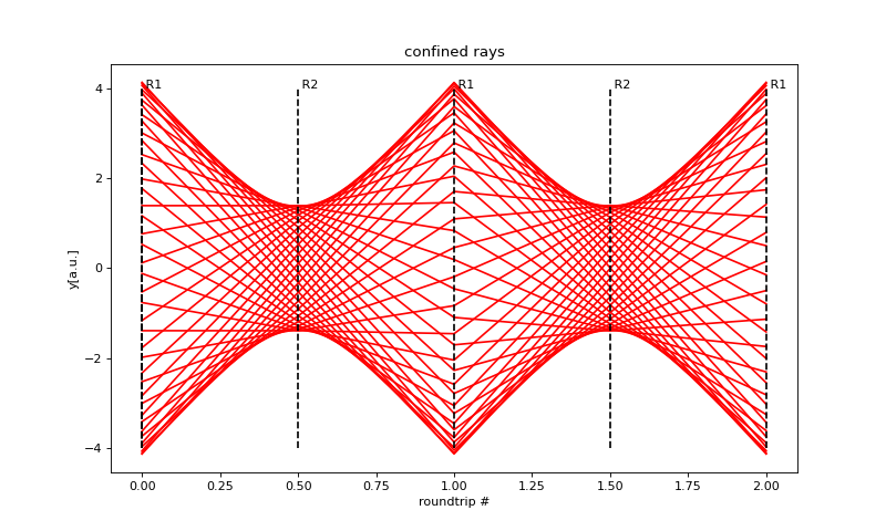
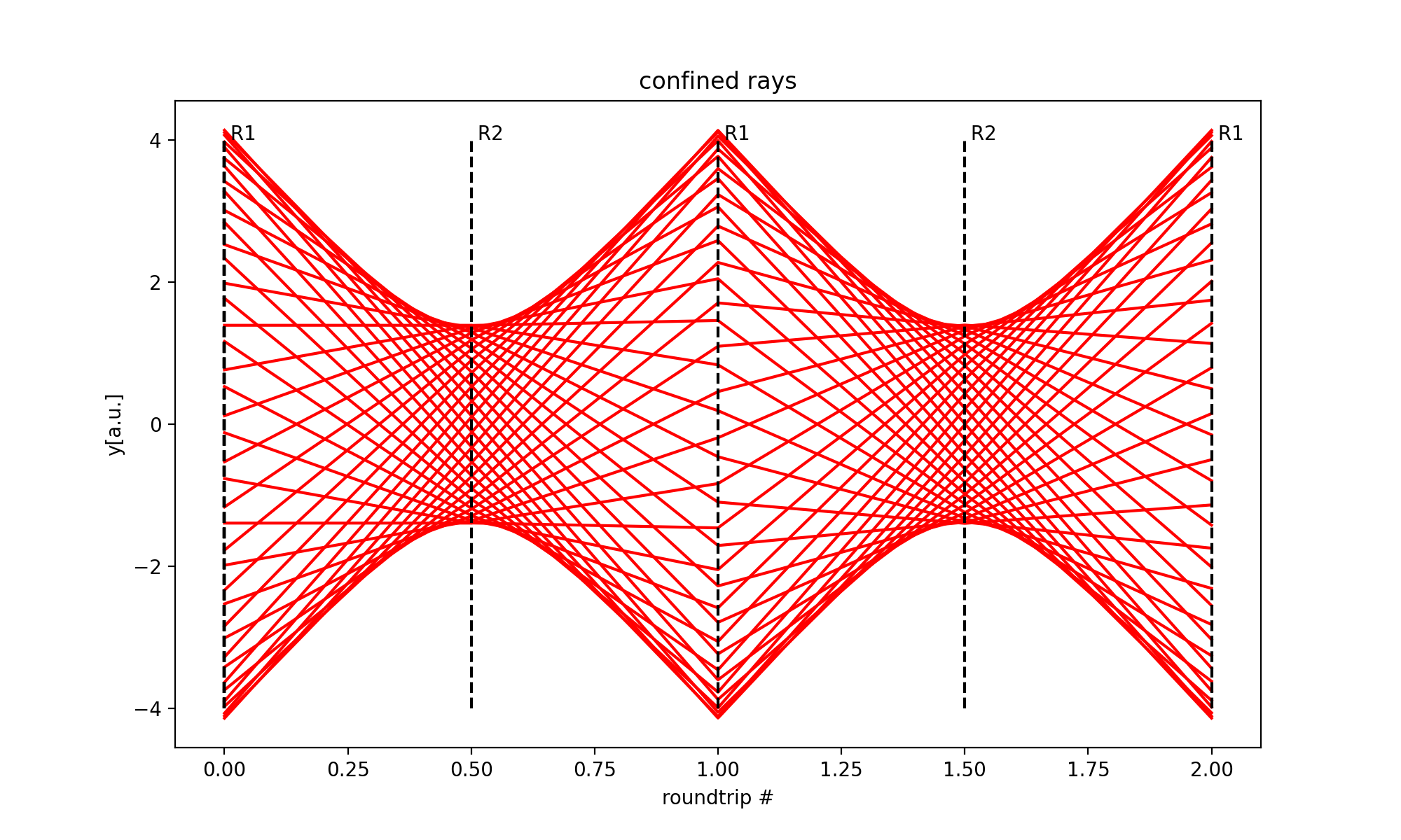
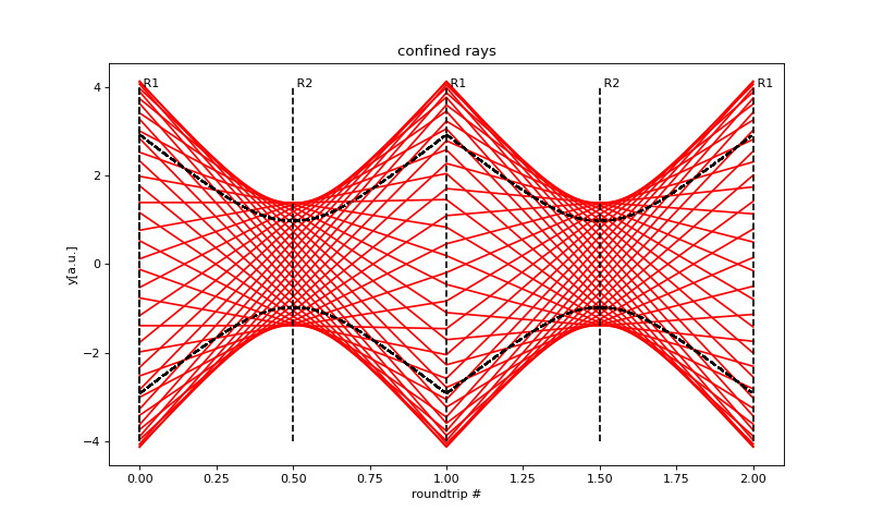
In the following Python script we calculate the propagation of a large number of rays in the resonator.

(Source code, png, hires.png, pdf)

7.5.8.4. Second moments

The envelope of the bundle of rays and other parameters can be found using second moments.

For the input rays:

\[\begin{split}\mathbf{R}_0=\begin{bmatrix}y_0 \\ \theta_0\\ \end{bmatrix} =2c\begin{bmatrix} z_1\cos(\alpha)-z_R\sin(\alpha) \\ \cos(\alpha) \\ \end{bmatrix}\;0 \leq \alpha \leq 2\pi\end{split}\]

we find for the second moment of \(y_0\):

\[\langle{y_0^2}\rangle=\frac{1}{2\pi}\int_0^{2\pi}y_0(\alpha)^2\mathrm{d}\alpha=\frac{4c^2}{2\pi}\int_0^{2\pi}(z_1\cos\alpha-z_R\sin\alpha)^2\mathrm{d}\alpha=\]

\[=\frac{4c^2}{2\pi}\left[z_1^2\int_0^{2\pi}\cos^2\alpha\mathrm{d}\alpha+z_R^2\int_0^{2\pi}\sin^2\alpha\mathrm{d}\alpha-2z_1z_R\int_0^{2\pi}\sin\alpha\cos\alpha\mathrm{d}\alpha\right]=\]

\[=\frac{4c^2}{2\pi}\left[\pi{z_1^2}+\pi{z_R^2}+0\right]=2c^2\left(z_1^2+z_R^2\right)\]

In a similar way we find for the second moments of \(\theta_0\) and \(y_0\theta_0\):

\[\langle{\theta_0^2}\rangle=\frac{1}{2\pi}\int_0^{2\pi}\theta_0(\alpha)^2\mathrm{d}\alpha=2c^2\]

\[\langle{y_0\theta_0}\rangle=\frac{1}{2\pi}\int_0^{2\pi}{y_0}(\alpha)\theta_0(\alpha)\mathrm{d}\alpha=2c^2z_1\]

In general we want to know the rays at a distance \(z'\) from the input-reference plane:

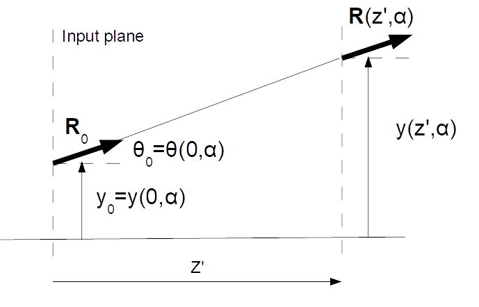
In other words we want to know \(\mathbf{R}(z',\alpha)\) for a given input ray \(\mathbf{R}_0=\mathbf{R}(0,\alpha)\) The ray at a distance \(z'\) can be found by propagating in free space (refractive index = 1):

\[\begin{split}\mathbf{R}(z',\alpha)=\begin{bmatrix} 1 & z' \\ 0 & 1 \\ \end{bmatrix}\mathbf{R}_0= \begin{bmatrix} y_0 + z'\theta_0 \\ \theta_0 \\ \end{bmatrix}= 2c\begin{bmatrix} z_1\cos{\alpha}-z_R\sin{\alpha}+z'\theta_0 \\ \theta_0 \\ \end{bmatrix}\end{split}\]

Using \(\theta_0=\cos{\alpha}\) and \(z \equiv{z_1+z'}\) we find for the rays at a distance, \(z\), from the beam waist (at a distance \(z_1\) from the reference plane):

\[\begin{split}\mathbf{R}(z,\alpha)=2c\begin{bmatrix} z\cos{\alpha}-z_R\sin{\alpha} \\ \cos{\alpha} \\ \end{bmatrix}\end{split}\]

The second moments at \(z\) are now:

\[\begin{split}\langle{y(z)^2}\rangle=2c^2(z^2+z_R^2)\equiv{w(z)^2}\\ \langle\theta(z)^2\rangle=2c^2\\ \langle{y(z)}\theta(z)\rangle=2c^2z\end{split}\]

With \(w_0\equiv{w(0)}=\sqrt{2}cz_R\) we define the beam waist \(w_0\) at \(z=0\). The size of the beam at a distance, \(z\), from the waist is:

\[w(z)^2=2c^2z_R^2\left(1+\frac{z^2}{z_R^2}\right)\]

or:

\[w(z)^2=w_0^2\left(1+\frac{z^2}{z_R^2}\right)\]

This formula of the size of the beam (bundle of confined rays) is exactly the same as the formula of the beam size of a Gaussian beam modelled according to the theory of physical optics, based on Maxwell’s equations. Also, the beam-area doubles when propagating a distance, \(z_R\), from the waist:

\[w(z_R)^2=2c^2z_R^2(1+1)=2w_0^2\]

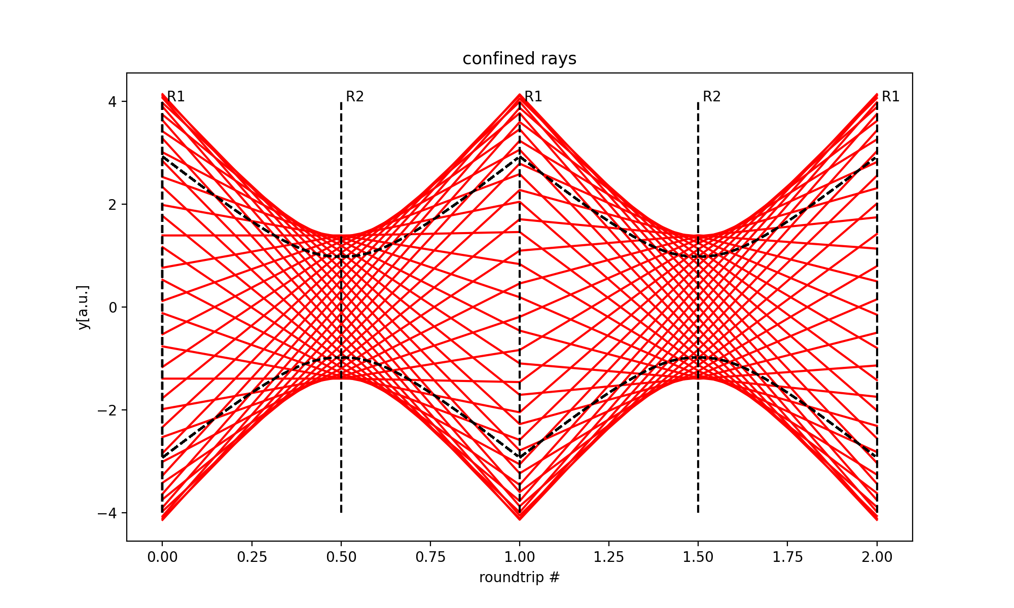
according to the definition of the Rayleigh length. The beam size, \(w(z)\), is also plotted in the figure below executing the same Python script as before but now with the second moments included (black dashed curves).

(Source code, png, hires.png, pdf)

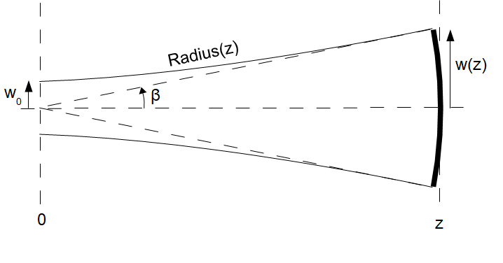
7.5.8.5. Wavefront radius

The radius of the wavefront can be found as follows: From the figure it follows that:

\[\beta=\frac{dw(z)}{dz}=\frac{w(z)}{Radius(z)}\]

\[\frac{dw(z)^2}{dz}=2w\frac{dw}{dz}=2w(z)\frac{w(z)}{Radius(z)}=2\frac{\langle{y(z)^2}\rangle}{Radius(z)}\]

Also:

\[\frac{d{w(z)^2}}{dz}=\frac{d}{dz}[2c^2(z^2+z_R^2)]=4c^2z=2\langle{y(z)}\theta(z)\rangle\]

So, we find for the radius of the wavefront at large values of z:

\[Radius(z)=\frac{\langle{y(z)^2}\rangle}{\langle{y(z)\theta(z)}\rangle}=\frac{w_0^2(1+\frac{z^2}{z_R^2})}{2c^2z} =\frac{2c^2(z^2+z_R^2)}{2c^2z}=z(1+\frac{z_R^2}{z^2})\]

7.5.8.6. Brightness

The following parameter, called the Brightness of the beam, does not change while propagating the beam:

\[Brightness\equiv\sqrt{\langle{y(z)^2}\rangle\langle\theta{(z)^2}\rangle-\langle{y(z)}\theta(z)\rangle^2} =\sqrt{4c^4(z^2+z_R^2-z^2)}=2c^2z_R=const\]

7.5.8.7. Get the constant \(c\)

The constant \(c\) is still unknown and can be obtained by using Heisenberg’s uncertainty relation or by comparing the results with the formulas obtained using physical optics, the solution of the wave equation.

a) Heisenberg:

The angle, \(\beta\), is given by:

\[\beta= \frac{w(z)}{z}\mid_{z\rightarrow\infty}=\frac{w_0\frac{z}{z_R}}{z}=\frac{w_0}{z_R}\]

The Heisenberg relation for the uncertainty of the impulse and position in the transverse direction, \(y\), of a photon is given by:

\[\Delta{P_y}\Delta{y}=h\]

Assume that the uncertainty of the impulse, \(p_z=\frac{h}{\lambda}\), \(\Delta{p_z}\) in the z direction is zero, the angle, \(\beta\) is also given by:

\[2\beta=\frac{\Delta{p_y}}{p_z}=\frac{\frac{h}{2w_0}} {\frac{h}{\lambda}}=\frac{\lambda}{2w_0}\]

So, from:

\[2\beta=\frac{2w_0}{z_R}=\frac{\lambda}{2w_0}\]

it follows that:

\[ \begin{align}\begin{aligned}4w_0^2=\lambda{z_R}\\8c^2z_R^2=\lambda{z_R}\end{aligned}\end{align} \]

The constant, \(c\) is:

\[c=\frac{\lambda}{4\sqrt{2}w_0}\]

b) Compare with physical optics solution:

For a round beam the Rayleigh length is:

\[z_R=\frac{\pi{w_0^2}}{\lambda}\]

using \(z_R=\frac{w_0}{\sqrt{2}c}\) we find for the constant \(c\):

\[c=\frac{\lambda}{\pi{\sqrt{2}w_0}}\]

(There is a slight difference with the Heisenberg method. Maybe this is due to the slab geometry versus cylinder geometry? Comments are welcome!)